Finding region boundaries

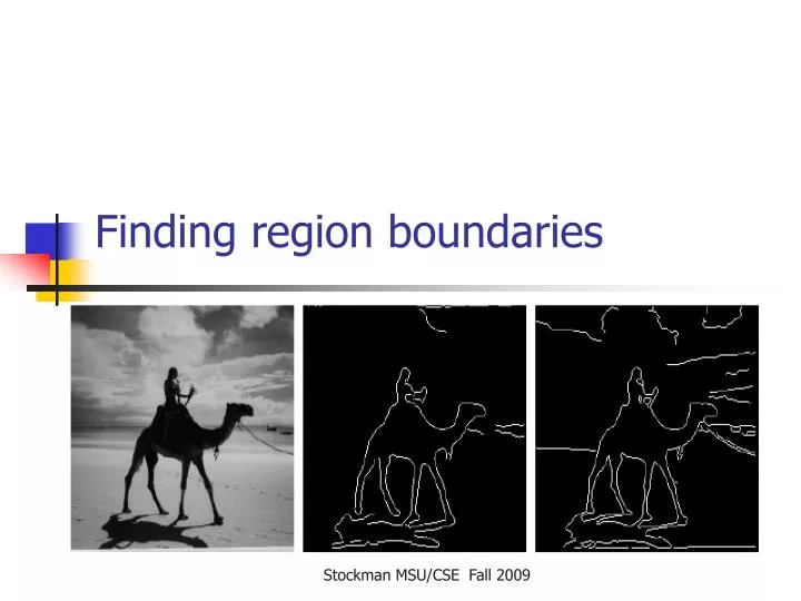
1. Finding region boundaries Stockman MSU/CSE Fall 2009

2. Object boundaries • How to detect? • How to represent? • Problems relative to region/area segmentation Stockman MSU/CSE Fall 2009

3. advantages • Contrast often more reliable under varying lighting • Boundaries give precise location • Boundaries have useful shape information • Boundary representation is sparse • Humans use edge information Stockman MSU/CSE Fall 2009

4. problems • Detection weakens at boundary corners • Topology of result is imperfect Stockman MSU/CSE Fall 2009

5. topics • Aggregating chains of boundary pixels • Line and curve fitting • Angles, sides, vertices • Ribbons • Imperfect graphs Stockman MSU/CSE Fall 2009

6. Canny edge detector/tracker • Detect, then follow high gradient boundary pixels • Track along a “thin” edge • Bridge across weaker contrast Stockman MSU/CSE Fall 2009

7. Canny algorithm data Stockman MSU/CSE Fall 2009

8. Overall Canny algorithm Stockman MSU/CSE Fall 2009

9. Create thin edge response by suppressing weaker neighbors • Find neighbors in direction of the gradient (across the edge) • If neighbor response is weaker, delete it. • Recall thick edges from 5x5 Sobel or Prewitt Stockman MSU/CSE Fall 2009

10. Begin tracking only at high gradient points Stockman MSU/CSE Fall 2009

11. Results with two spreads Stockman MSU/CSE Fall 2009

12. Notes/Variations • Very few parameters needed • Can use multiple spreads and correlate the results in multiple edge images • Can carefully manage the use of low and high thresholds, perhaps depending on size and quality of the current track • Canny edge tracker is very popular Stockman MSU/CSE Fall 2009

13. Aggregating pixels into curves Producing a discrete data structure with meaningful parts. Stockman MSU/CSE Fall 2009

14. Tracking tasks Canny algorithm does some of these. Stockman MSU/CSE Fall 2009

15. Possible output from tracker Stockman MSU/CSE Fall 2009

16. The Hough Transform Detecting a straight line segment as a cluster in rho-theta space. (Can do circles or ellipses too.) Stockman MSU/CSE Fall 2009

17. Voting evidence in cluster space Stockman MSU/CSE Fall 2009

18. Pixels with distinct (r,c) coordinates map to same (d, Θ) Y Detected set of edge points d Textbook coordinate system vs Cartesian system Θ X Stockman MSU/CSE Fall 2009

19. Mapping pixels (r, c) to polar parmameters (d, Θ) Row-column system Cartesian coordinate system d = x cos Θ + y sin Θ Stockman MSU/CSE Fall 2009

20. Simple algorithm overview Stockman MSU/CSE Fall 2009

21. Possible implementation Stockman MSU/CSE Fall 2009

22. Binning evidence: note that original pixels [R, C] are saved in the bins. Stockman MSU/CSE Fall 2009

23. Real world considerations • The gradient direction Θ is bound to have error (due to what?) • Since d is computed from Θ, d will also have error • Thus, evidence is spread in parameter space and may frustrate binning methods (2D histogram) Stockman MSU/CSE Fall 2009

24. Solutions • Bins for (d, Θ) can be smoothed to aggregate neighbors. • Multiple evidence can be put into the bins by adding deltas to Θ and computing variations of (d, Θ) • Clustering can be done in real space; e.g. do not use binning • Busy images should be handled using a grid of (overlapping) windows to avoid a cluttered transform space Stockman MSU/CSE Fall 2009

25. What is the space of d and Θ ? • Many apps range Θ from 0 to π only • However, gradient direction can be detected from 0 to 2 π. • Imagine a checkerboard – there are 4 prominent directions, not 2. • Using full range of direction requires negative values of d – consider checkerboard with origin in the center. Stockman MSU/CSE Fall 2009

26. Additional material • Plastic slides from Stockman • Plastic slides from Kasturi Stockman MSU/CSE Fall 2009

27. Image to map work of Kasturi Stockman MSU/CSE Fall 2009

28. Circular Hough Transform There are 3 parameters for a circle Stockman MSU/CSE Fall 2009

29. Possible implementation Stockman MSU/CSE Fall 2009

30. Some notes • Circular and elliptical Hough Transforms are interesting, but of dubious value by themselves • Smarter tracking methods, such as Snakes, balloons, etc. might be needed along with region features • There are weak publications that will not help in real applications. Stockman MSU/CSE Fall 2009

31. Fitting models to edge data Can use straight line segments for data compression, or parametric curves for shape detection. Stockman MSU/CSE Fall 2009

32. Fitting curves Stockman MSU/CSE Fall 2009

33. An unlimited number of models Stockman MSU/CSE Fall 2009

34. Least squares fitting Stockman MSU/CSE Fall 2009

35. Best fit minimizes sum of squared errors Stockman MSU/CSE Fall 2009

36. Stockman MSU/CSE Fall 2009

37. Axis of least inertia better? Stockman MSU/CSE Fall 2009

38. Ramer’s alg: perimeter to polygon Stockman MSU/CSE Fall 2009

39. Angles, corners, ribbons Stockman MSU/CSE Fall 2009

40. The downspout as a ribbon Stockman MSU/CSE Fall 2009

41. Road and canal as ribbons Stockman MSU/CSE Fall 2009

42. More boundary detection later • Will investigate “physics-based models” • Can fit to 2D (snakes) or 3D data (balloons) • Models do not allow the object topology to break • Models enforce object smoothness Stockman MSU/CSE Fall 2009