Download
1 / 29
290 likes | 469 Views
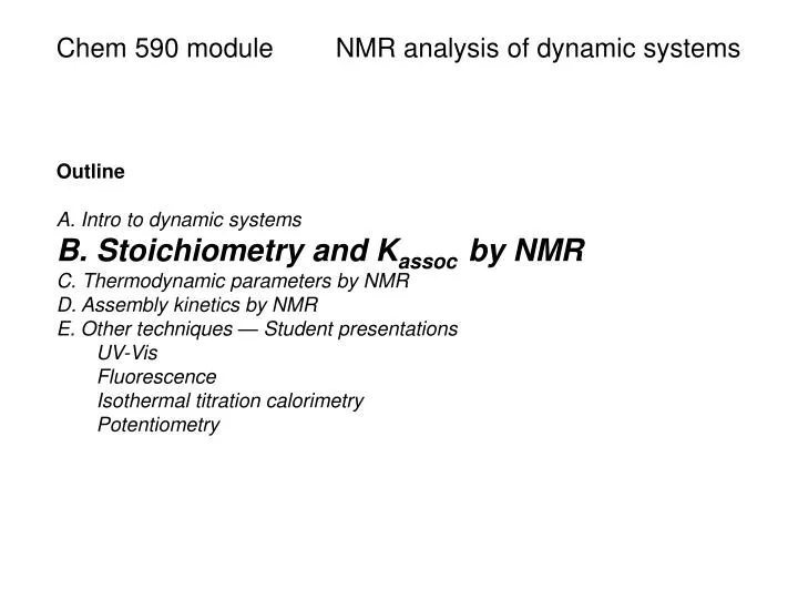
Chem 590 module NMR analysis of dynamic systems Outline A. Intro to dynamic systems B . Stoichiometry and K assoc by NMR C . Thermodynamic parameters by NMR D. Assembly kinetics by NMR E. Other techniques — Student presentations UV-Vis Fluorescence

E N D
Chem 590 module NMR analysis of dynamic systems Outline A. Intro to dynamic systems B. Stoichiometry and Kassocby NMR C. Thermodynamic parameters by NMR D. Assembly kinetics by NMR E. Other techniques — Student presentations UV-Vis Fluorescence Isothermal titration calorimetry Potentiometry
Learning Aims A. Become familiar with dynamic systems and the meanings of the quantities used to characterize them. B1. De-mystify the black-box of Kassoc determinations by all methods. B2. Obtain in-depth understanding of the math and models for 1:1 binding equilibria. B3. Understand the mathematics of the 1:1 binding isotherm, its applications, and its limitations. B4. Gain a comprehensive understanding of how d arises when looking at dynamic systems. B5. Get practical, step-by-step instructions for determining stoichiometry and Kassoc by NMR. C. Learn how NMR can be used to determine ∆H and ∆S for a given equilibrium D. Achieve a beginner-level understanding of studying kinetics by NMR. The goal is to allow you to understand literature, not to teach you how to do the experiments. E. Get a beginner-level understanding of other methods for determining Kassoc UV-Vis, Fluorescence, Isothermal titration calorimetry, Potentiometry
Dynamic systems are driven by weak interactions – + Electrostatic interactions Dispersive forces Hydrogen bonds Aromatic-aromatic interactions and cation-pi interactions The hydrophobic effect Ion–Dipole interactions – – + + Dipole–Dipole interactions
A complex metal-ligand assembly 6 H4L + 4 Ga(acac)3 + 12 KOH + 12 Et4NCl K5[Et4N]7[Ga4L6] (+ H2O, KCl, etc) H4L [Ga4L6]12–
A chiral guest allows resolution into enantiomeric cages Et4N@[Ga4L6] + nicotine@[Ga4L6] nicotine@ ∆∆∆∆-[Ga4L6] Guest exchange Resolution of diastereomers Exchange back to achiral guest without loss of host chirality Et4N@ ∆∆∆∆-[Ga4L6]
Exchange of L1 for L2 occurs without complete disassembly Et4N@ ∆∆∆∆-[Ga4L16] + 6 L2 Et4N@ ∆∆∆∆-[Ga4L26] + 6 L1
Cation-π interactions: Factor Xa – inhibitor binding Aromatic cage S4 pocket -lined by aromatic residues Kd= 0.28 M Kd= 29 M
Lysozyme mutants fold more weakly when hydrophobic groups are shrunk down to Ala ∆∆G correlates with hydrophobic (interfacial) surface area! 15-20 cal/mol for each Å2
Cyclodextrin hosts bind hydrophobic guests with different contributions from ∆H and T∆S
Rates of exchange and NMR N-methylformamide(left) and methyl formate (right) in CDCl3 at 90 MHz
Calculated barriers to rotation trans cis trans HF 3-21G (Gas phase) trans cis
Rates change as a function of temperature Variable temperature NMR of DMF
Slow exchange: integration to determine complex stoichiometry * * Integration of methoxy (*) and adamantane (•) signals gave a 4:1 molar ratio. (Later confirmed by X-ray)
A Practical Guide — Job plot sample prep 1. Prepare stocks [A stock] = 5 mM [B stock] = 5 mM 2. Create samples with fixed [At + Bt] as below: cA cA•∆d 3. Record Dd, calculate Dd•cA, Plot as shown at right
Diffusion-Ordered SpectroscopY (DOSY) Stokes-Einstein relationship: D = kT / 6πhRH D = diffusion coefficient k = Boltzmann constant h= solvent viscosity RH = hydrodynamic radius, which can be related to MW by calibration on related molecules
A system in fast exchange – real data for dfree and dbound [peptide]t = 1 mM
Hypothetical curves for f11 vs. conc. plots based on the generalized 1:1 binding isotherm
Exemplary NMR Titration Data Average Kassoc = 180 M–1 Schalley et al. Chem. Eur. J.2003, 9, 1332.
A Practical Guide — Sample preparation Choose starting concentrations 1. Prepare 5 mL of stock A 2. Remove 0.6 mL of stock and put in NMR tube 3. Calculate amount of B needed to make 4 mL of B at 30x [A] 4. Weigh that amount of B into vial, and dissolve in 4 mL of stock A 5. Transfer that titrant into a gas-tight 100 or 250 uL syringe All of this ensures that Atstays constant throughout titration. 1. 2. 3. 4.
A Practical Guide — Titration Record NMR to determine dfree Add 10 uL of titrant Record NMR again Repeat… Hints: -You want to observe a significant Dd with each addition. You want lots of data points on the curved part of the isotherm. You want to get as close to saturation as possible. This will require making judgments on the fly and increasing the amount you add as you go along. It is not unusual for the increments to start at 10 uL and to be 250 uL by the end of the titration. - Mix well at each addition (invert >5 times). Mixing is slow in a narrow NMR tube.
A Practical Guide — Data Analysis 1. In a spreadsheet, record dobs and total volume of titrant added for each spectrum. 2. Convert to the y and x values needed for plotting, Ddobs and Bt. 3. Input these two columns of data into Origin. 4. Fit to the 1:1 binding isotherm to determine the parameters Ddmax and Kassoc. Be sure to try a few different initial guesses. Be sure to check the quality of fit. If you haven’t already done so, confirm stoichiometry by Job plot or other method.
Exemplary Data — van’t Hoff Plots Normally 4-5 values for T are enough RafaellaFaraoni, PhD thesis, ETH Zurich
Exemplary Data — Very Slow Exchange Kinetics Exchange of guest P (complex 1•P•1; triangles) for guest A (complex 1•A•1;squares) was followed over 4 hours taking a new NMR measurement every 5 minutes. Rebek et al. Proc. Nat. Acad. Sci. USA1999, 96, 8344.
NMR Line-Shape Analysis At a given temperature where intermediate exchange is observed, k = k1 + k–1 can be determined by fitting: • A = intensity of NMR signal (y axis) • = frequency (x axis) • M0 = some magnetization constant, determined in a separate experiment • W1 = wobs–w0 for signal 1 (offset) • W2 = wobs–w0 for signal 2 (offset)
Exemplary Data — NMR Line-Shape Analysis - Red traces are fitted curves, black traces are actual data. - There is a built-in module in TOPSPIN that does this fitting (CG?). k ~ 3500 s–1 k = 735 s–1 k = 17.5 s–1
Exemplary EXSY data for guest exchange “Meout” “Mein” Integrate 3D on-axis peaks and cross peaks to obtain k1 and k–1 See Perrin, C. L.; Dwyer, T. J. Chem. Rev. 1990, 90, 935-967 for a review