Section 4.7 Optimization Problems

1. Applications of Differentiation Section 4.7Optimization Problems

2. Applications of Differentiation • The methods we have learned in this chapter for finding extreme values have practical applications in many areas of life. • A business person wants to minimize costs and maximize profits. • A traveler wants to minimize transportation time. • Fermat’s Principle in optics states that light follows the path that takes the least time.

3. Optimization Problems • In this section we solve such problems as: • Maximizing areas, volumes, and profits • Minimizing distances, times, and costs

4. Optimization Problems • In solving such practical problems, the greatest challenge is often to convert the word problem into a mathematical optimization problem—by setting up the function that is to be maximized or minimized. • Thus, there are six steps involved in solving optimization problems. • These are as follows.

5. Steps in SolvingOptimization Problems

6. 1. Understand the Problem • Read the problem carefully until it is clearly understood. • Ask yourself: • What is the unknown? • What are the given quantities? • What are the given conditions?

7. 3. Introduce Notation • Assign a symbol to the quantity that is to be maximized or minimized. • Let’s call it Q for now. 2. Draw a Diagram • In most problems, it is useful to draw a diagram and identify the given and required quantities on the diagram.

8. 4. Express Q in terms of the variables • Express Q in terms of some of the other symbols from Step 3. 3. Introduce Notation • Also, select symbols (a, b, c, . . . , x, y)for other unknown quantities and label the diagram with these symbols. • It may help to use initials as suggestive symbols. • Some examples are: A for area, h for height, and t for time.

9. 5. Express Q in terms of one variable • If Q has been expressed as a function of more than one variable in Step 4, use the given information to find relationships—in the form of equations—among these variables. • Then, use the equations to eliminate all but one variable in the expression for Q. • Thus, Q will be expressed as a function of one variable x, say, Q =f (x). • Write the domain of this function.

10. 6. Find the Abs. Max./Min of f • Use the methods of Sections 4.1 and 4.3 to find the absolute maximum or minimum value of f. • In particular, if the domain of f is a closed interval, then the Closed Interval Method in Section 4.1 can be used.

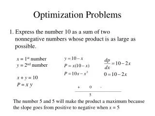
11. Optimization Problems – Ex. 1 • A farmer has 2400 ft of fencing and wants to fence off a rectangular field that borders a straight river. He needs no fence along the river. • What are the dimensions of the field that has the largest area? • In order to get a feeling for what is happening in the problem, let’s experiment with some special cases.

12. Optimization Problems – Ex. 1 • Here are three possible ways of laying out the 2400 ft of fencing.

13. Optimization Problems – Ex. 1 • We see that when we try shallow, wide fields or deep, narrow fields, we get relatively small areas. • It seems plausible that there is some intermediate configuration that produces the largest area.

14. Optimization Problems – Ex. 1 • The figure illustrates the general case. • We wish to maximize the area A of the rectangle. • Let x and y be the depth and width of the rectangle (in feet). • Then, we express A in terms of x and y: A = xy

15. Optimization Problems – Ex. 1 • We want to express A as a function of just one variable. • So, we eliminate y by expressing it in terms of x. • To do this, we use the given information that the total length of the fencing is 2400 ft. • Thus, 2x +y = 2400

16. Optimization Problems – Ex. 1 • From that equation, we have: y = 2400 – 2x • This gives: A = x(2400 – 2x) = 2400x - 2x2 • Note that x ≥ 0 and x ≤ 1200 (otherwise A < 0).

17. Optimization Problems – Ex. 1 • So, the function that we wish to maximize is: A(x) = 2400x – 2x2 0 ≤x ≤ 1200 • The derivative is: A’(x) = 2400 – 4x • So,to find the critical numbers, we solve: 2400 – 4x = 0 • This gives: x = 600 • There are no singular points.

18. Optimization Problems – Ex. 1 • The maximum value of A must occur either at that critical number or at an endpoint of the interval. • A(0) = 0; A(600) = 720,000; and A(1200) = 0 • So, the Closed Interval Method gives the maximum value as: A(600) = 720,000

19. Optimization Problems – Ex. 1 • Alternatively, we could have observed that A’’(x) = – 4 < 0 for all x • So, A is always concave downward and the local maximum at x = 600 must be an absolute maximum.

20. Optimization Problems – Ex. 1 • Thus, the rectangular field should be: • 600 ft deep • 1200 ft wide

21. Optimization Problems – Ex. 2 • A cylindrical can is to be made to hold 1 L of oil. • Find the dimensions that will minimize the cost of the metal to manufacture the can.

22. Optimization Problems – Ex. 2 • Draw the diagram as in this figure, where r is the radius and h the height (both in centimeters).

23. Optimization Problems – Ex. 2 • To minimize the cost of the metal, we minimize the total surface area of the cylinder (top, bottom, and sides.)

24. Optimization Problems – Ex. 2 • We see that the sides are made from a rectangular sheet with dimensions 2πr and h.

25. Optimization Problems – Ex. 2 • So, the surface area is:A = 2πr2+ 2πrh

26. Optimization Problems – Ex. 2 • To eliminate h, we use the fact that the volume is given as 1 L, which we take to be 1000 cm3. • Thus, πr2h =1000 • This gives h =1000/(πr2)

27. Optimization Problems – Ex. 2 • Substituting this in the expression for A gives: • So, the function that we want to minimize is:

28. Optimization Problems – Ex. 2 • To find the critical numbers, we differentiate: • Then, A’(r) = 0 when πr3 = 500 • So, the only critical number is:

29. Optimization Problems – Ex. 2 • As the domain of A is (0,), we can’t use the argument of Example 1 concerning endpoints. • However, we can observe that A’(r) < 0 for and A’(r) > 0 for • So, A is decreasing for all r to the left of the critical number and increasing for all r to the right. • Thus, must give rise to an absoluteminimum.

30. Optimization Problems – Ex. 2 • Alternatively, we could argue that A(r) → ∞ as r → 0+ and A(r) → ∞ as r → ∞. • So, there must be a minimum value of A(r), which must occur at the critical number.

31. Optimization Problems – Ex. 2 • The value of h corresponding to is:

32. Optimization Problems – Ex. 2 • Thus, to minimize the cost of the can, • The radius should be cm • The height should be equal to twice the radius—namely, the diameter.

33. Remark 1 • The argument used in the example to justify the absolute minimum is a variant of the First Derivative Test—which applies only to local maximum or minimum values. • It is stated next for future reference.

34. First Deriv. Test for Abs. Extrema • Suppose that c is a critical number of a continuous function f defined on an interval. • If f’(x) > 0 for all x <c and f’(x) < 0 for all x > c, then f(c) is the absolute maximum value of f. • If f’(x) < 0 for all x <c and if f’(x) > 0 for all x > c, then f(c) is the absolute minimum value of f.

35. Remark 2 • An alternative method for solving optimization problems is to use implicit differentiation. • Let’s look at the example again to illustrate the method.

36. Implicit Differentiation • We work with the same equations A = 2πr2 + 2πrh πr2h = 100 • However, instead of eliminating h, we differentiate both equations implicitly with respect to r : A’ = 4πr + 2πh + 2πrh’ 2πrh + πr2h’ = 0

37. Implicit Differentiation • The minimum occurs at a critical number. • So, we set A’ = 0, simplify, and arrive at the equations 2r +h +rh’ = 0 2h +rh’ = 0 • Subtraction gives: 2r - h = 0 or h = 2r

38. Optimization Problems – Ex. 3 • Find the point on the parabola y2 = 2x that is closest to the point (1, 4).

39. Optimization Problems – Ex. 3 • The distance between the point (1, 4) and the point (x, y) is: • However, if (x, y) lies on the parabola, then x = ½ y2. • So, the expression for d becomes:

40. Optimization Problems – Ex. 3 • Alternatively, we could have substituted to get d in terms of x alone.

41. Optimization Problems – Ex. 3 • Instead of minimizing d, we minimize its square: • You should convince yourself that the minimum of d occurs at the same point as the minimum of d 2. • However, d 2 is easier to work with.

42. Optimization Problems – Ex. 3 • Differentiating, we obtain: • So, f’(y) = 0 when y = 2.

43. Optimization Problems – Ex. 3 • Observe that f’(y) < 0 when y < 2 and f’(y) > 0 when y > 2. • So, by the First Derivative Test for Absolute Extreme Values, the absolute minimum occurs when y = 2. • Alternatively, we could simply say that, due to the geometric nature of the problem, it’s obvious that there is a closest point but not a farthest point.

44. Optimization Problems – Ex. 3 • The corresponding value of x is: x = ½ y2 = 2 • Thus, the point on y2 = 2x closest to (1, 4)is (2, 2).

45. Optimization Problems – Ex. 4 • A man launches his boat from point A on a bank of a straight river, 3 km wide, and wants to reach point B (8 km downstream on the opposite bank) as quickly as possible.

46. Optimization Problems – Ex. 4 • He could proceed in any of three ways: • Row his boat directly across the river to point C and then run to B • Row directly to B • Row to some point D between C and B and then run to B

47. Optimization Problems – Ex. 4 • If he can row 6 km/h and run 8 km/h, where should he land to reach B as soon as possible? • We assume that the speed of the water is negligible compared with the speed at which he rows.

48. Optimization Problems – Ex. 4 • If we let x be the distance from C to D, then: • The running distance is: |DB| = 8 – x • The Pythagorean Theorem gives the rowing distance as: |AD| =

49. Optimization Problems – Ex. 4 • We use the equation • Then, the rowing time is: • The running time is: (8 – x)/8 • So, the total time T as a function of x is:

50. Optimization Problems – Ex. 4 • The domain of this function T is [0, 8]. • Notice that if x = 0, he rows to C, and if x = 8, he rows directly to B. • The derivative of T is: