Download
1 / 33
330 likes | 487 Views
C-H plane analysis of plasma turbulence in SSX and LAPD. Last updated 6/20/14 by Peter Weck. Contents. Complexity -entropy planes for full datasets Helicity dependence of SSX complexity-entropy plane SSX complexity -entropy planes for varied embedding delay

E N D
C-H plane analysis of plasma turbulence in SSX and LAPD Last updated 6/20/14 by Peter Weck
Contents Complexity-entropy planes for full datasets Helicitydependence of SSX complexity-entropy plane SSX complexity-entropy planes for varied embedding delay Dependence of SSX complexity-entropy plane on time window
Section I Complexity-entropy planes for full datasets
The CH Plane Figure 1: SSX points are averages over 12 channels, all 3 directions, and ~40 shots for two helicity settings. LAPD points are averages over 25 runs at two positions. Error bars represent standard deviations in C and PE, below and above averages.
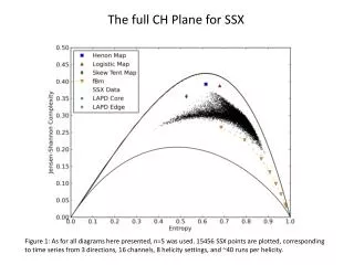
The full CH Plane for SSX Figure 2: As for all diagrams here presented, n=5 was used. 15456 SSX points are plotted, corresponding to time series from 3 directions, 16 channels, 8 helicity settings, and ~40 runs per helicity.
The SSX CH Plane, first 12 channels only Figure 3: 11592 SSX points are plotted, corresponding to time series from 3 directions, 12 channels, 8 helicity settings, and ~40 runs per helicity.
The Full CH Plane for LAPD Figure 4: 775 LAPD points are plotted, corresponding to time series from 25 runs and 31 positions.
Section II Helicitydependence of SSX complexity-entropy plane
All SSX data for each helicity setting: unstuffed 0.1 mWb 0.25 mWb 0.5 mWb
All SSX data for each helicity cont. 0.75mWb 1.0 mWb 1.25 mWb 1.5 mWb
SSX CH Plane, averaged over shots (channel 1 of 16) Figure 5: Note that points represent the radial direction, plus signs theta, and x-marks z. The color scale represents helicity.
SSX CH Plane, averaged over shots and directions (channel 1 of 16) Figure 6: The color scale again represents helicity. Note the loop executed in the right side of the plane as helicity is varied. The least entropic helicity setting (pale blue) appears to be 0.5mWb.
SSX CH Plane, averaged over shots and directions (channel 6 of 16) Figure 7: The same looping behavior as in Figure 6 seems to occur for channel 6 data, although the loop is angled a little higher in the plane
SSX CH Plane, averaged over shots and directions (channel 12 of 16) Figure 8: Channel 12 data seems to loop through an even higher complexity region of the CH plane. Once again, 0.5mWb has the lowest entropy point.
Section III Complexity-entropy planes for varied embedding delay
The following two slides show SSX data up to channel 12 for various embedding delays. • While τ denotes use of the embedding delay as described in most of the literature, which effectively reduces the length of the analyzed series by a factor of τ, τ’ indicates that a delay analysis like that used for the increments method was applied. • So τ ’ analyzed series are kept significantly longer, only losing (n-1) τ ’ or so values. • Figure 3 (τ ’ = τ = 1) has been reproduced above to provide comparison with the diagrams to follow. • I was surprised to see that keeping more of the series actually lowered the overall complexity of SSX data, according to these diagrams.
τ = 2 τ = 4 τ = 6 τ = 8
τ ’ = 2 τ ’ = 4 τ ’ = 6 τ ’ = 8
Section IV Dependence of SSX complexity-entropy plane on time window
The following six slides show the full range of SSX data on the CH plane for six different 20 μs windows. • The data seems to drop further towards the rightmost corner of the plane the farther out in the time series you go, with 30-50 μs and 40-60 μs data occupying the upper/middle region of the plane and the 80-100 μs data closest to the PE=1, C=0 corner. • The same six plots were generated for embedding delays τ = 2, 4, 6, and 8 and τ ’ = 2, 4, 6, and 8, but I did not include them since introducing a delay seemed to have the same qualitative effect on all time windows as was seen for the 40-60 μs window data in the previous section (i.e. delays of τ’ = τ = 2 pulled the data closer to noise, and delays of 4, 6, and 8 pulled it up into higher regions of the plane).
The next six slides show CH planes with unstuffed and 0.5 mWb SSX data for six different 20 μs windows. • On each slide, the full range of the 0.5 mWb data up to channel 12 is shown top-left, the range of the unstuffed data up to channel 12 top-right, and the average position and standard deviations for both data sets bottom-center. • The 30-50 μs, 50-70 μs, and 40-60 μs window diagrams all seem fairly similar, with comparable positions and deviations for both unstuffed and 0.5 mWb settings. • The three windows after these ranges, however, drop the data dramatically towards the PE=1, C=0 corner of the plane. Latter portions of the time series also break the pattern of lower entropies for the 0.5 mWb setting which has consistently held for earlier portions of the time series.