Download
1 / 59
660 likes | 1.54k Views
Topic 4. Statistical Process Control (Control Charts) and Acceptance Sampling. Statistical Process Control. I. Statistical Process Control: graphical presentation of samples of process output over time used to monitoring (production) process and detect quality problems.

E N D
Topic 4. Statistical Process Control (Control Charts) and Acceptance Sampling
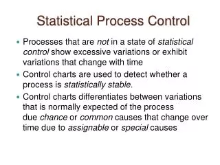
Statistical Process Control I. Statistical Process Control: • graphical presentation of samples of process output over time • used to monitoring (production) process and detect quality problems
Two Types of Variations • Nature vs. Assignable Variations
Idea Behind Control Charts • If (production) process is normal • only natural variations exist • samples of output is Normally distributed • within 3 std. 99.7% of time • Therefore, • If not within 3 std. ==> assignable variations exist! • UCL (Upper Control Limit) and LCL (Lower Control Limit) are set to correspond to the 3 std. lines if no specification
In control Signals • In control: plots Normally distributed, unbiased, no patterns • indicating no assignable variations exist
Out of control Signals • one plot outside UCL or LCL (for all charts) • 2 of 3 consecutive plots out of 2 std. Line (for X-bar chart) • 7 consecutive plots on one side (for X-bar chart) • indicating assignable variations exist, sign of quality problems.
Types of control chart • Variable Charts: for continuous quality measure • X-bar ( ) chart: process average • R chart: process dispersion and variation • Attribute Charts: for attribute quality measure • p chart: defective rate • c chart: number of defectives
Construct and Use Control Charts (X-bar Charts) • Construct X-bar chart • 1. based on some process information: If process (population) mean and standard deviation are known. • CL = • UCL = • LCL = • n: sample size • z: normal score (two tails), equals 3 without specification
Construct and Use Control Charts (X-bar Charts) • Some important normal scores • Z= 3 (99.7%) • Z= 2.5 (98.75%) • Z= 2.33 (98%) • Z= 2.17 (97%) • Z= 2 (95.5%) • Z= 1.96 (95%) • Z=1.645 (90%)
Construct and Use Control Charts (Example 1 for X-bar Chart by Method 1) • Example 1 • Samples taken from a process for making aluminum rods have an average of 2cm. The sample size is 16. The process variability is approximately normal and has a std. of 0.1cm. Design an X-bar chart for this process control.
Construct and Use Control Charts (X-bar Charts) • Construct X-bar Chart • 2. If process mean and standard deviation are unknown, X-bar Chart can be constructed based only on past samples • Assume k past samples with sample size n. • Sample i (i = 1, 2, …, k) has n observations • Sample mean for sample i is • Sample range for sample is
Construct and Use Control Charts (X-bar Charts) • 2. If process mean and standard deviation are unknown, X-bar Chart can be constructed based only on past samples (continuous) • The average of past k samples is • The range average of past k samples is
Construct and Use Control Charts(X-bar Chart) • 2. If process mean and standard deviation are unknown, X-bar Chart can be constructed based only on past samples (continuous) • X-bar chart is: • Mean factor is a function of sample size n
Construct and Use Control Charts (X-bar Chart) • 3. Differences between method 1. and method 2. • Method 1 is based known process (target or standard) information, while method 2 is based on past data information (target or standard unknown) • Therefore, if there is a out of control signal by method 1, we can say it is different from the target (standard). However, if there is a out of control signal by method 2, we cannot say it is different from the target (standard).
Construct and Use Control Charts (R Chart) • Construct R chart (based on past samples) are functions of sample size n
Construct and Use Control Charts (Example 2 for X-bar and R Charts by Method 2) • Example 2: • Five samples of drop-forged steel handles, with four observations in each sample, have been taken. The weight of each handle in the samples is given below (in ounces). Use the sample data to construct an X-bar chart and an R-chart to monitor the future process.
Construct and Use Control Charts (Example 2 for X-bar and R Charts by Method 2) • Continuous
Construct and Use Control Charts (Use X- bar chart and R chart) • Use X-bar chart and R chart • Calculate averages and ranges of new samples • Plot on the X-bar chart and R chart, respectively
Construct and Use Control Charts (Example 2 Continuous) • Five more samples of the handles are taken. Is the process in control (changed)?
Construct and Use Control Charts (p Chart) • Construct p chart (defective rate chart) based past samples • Assume there are k past samples with sample size n. • Each item in a sample may only have two possible outcomes: good or defective • In sample i (i = 1,2, …, k), there are number of defectives out of n items.
Construct and Use Control Charts (p Chart) • The defective rate for sample i is • The average number of defectives in past k samples is • And the average defective rate in the past samples is
Construct and Use Control Charts (p Chart) • P Chart is • Again, z is normal score (two tails)
Construct and Use Control Charts (p Chart) • Use p-chart • Calculate defective rates of new samples • Plot on the p-chart
Construct and Use Control Charts (Example 3 for p Chart) • Example 3 A good quality lawnmower is supposed to start at the first try. In the third quarter, 50 craftsman lawnmowers are started every day and an average of 4 did not start. In the fourth quarter, the number of lawnmower did not start (out of 50) in the first 6 days are 4, 5, 4, 6, 7, 6, respectively. Was the quality of lawnmower changed in the fourth quarter?
Construct and Use Control Charts (c Chart) • Only used when sample size is unknown • Number of complaints received in a postmaster office • Assume there are k past samples with unknown sample size • Sample i has number defectives • The average defective number in past samples is
Construct and Use Control Charts (c Chart) • c Chart is • Again, z is normal score (two tails)
Construct and Use Control Charts (c Chart) • Use c-chart • Count number of defectives in new samples • Plot on the c-chart
Construct and Use Control Charts (Example 4 for c Chart) • Example 4 • There have been complaints that the sports page of the Dubuque Register has lots of typos. The last 6 days have been examined carefully, and the number of typos/page is recorded below. Is the process in control?
Acceptance Sampling II. Acceptance Sampling • Acceptance Sampling: Accept or reject a lot (input components or finished products) based on inspection of a sample of products in the lot • Tool for Quality Assurance
Acceptance Sampling • Role of Inspection • Involved in all stages of production process • Inspection itself does not improve quality • Destructive and nondestructive inspection • Why sampling instead of 100% inspection? • Destructive test • Worker's morale • Cost consideration
Acceptance Sampling • Single Acceptance Sampling Plan: • Take a sample of size n from a lot with size N • Inspect the sample 100% • If number of defective > c, reject the whole lot; otherwise, accept it. • need to determine n and c.
Acceptance Sampling • Operating Characteristic (OC) Curves • to evaluate how well a single acceptance sampling plan discriminates between good and bad lots
Acceptance Sampling • Draw an OC curve approximately for a given n and c
Acceptance Sampling • Idea: • The number of defectives in a sample of size n with defective rate p follows a Poisson distribution approximately with parameter = n*p, when p is small, n is large, and N is even larger.
Acceptance Sampling • Procedure: • 1. Create a series of p = 1% to 10%. • 2. Calculate = n*p for each p. • 3. Use the Poisson table of Appendix B to find P(acceptance) for each and c. • 4. Link P(acceptance) to form a curve.
Acceptance Sampling • Example 5 for OC curve: A single sampling plan with n=100 and c=3 is used to inspect a shipment of 10000 computer memory chips. Draw the OC curve for the sampling plan.
Acceptance Sampling • Concepts related to the OC Curve • AQL: Acceptable quality level, the defective rate that a consumer is happy to accept (considers as a good lot) • LTPD: Lot tolerance percent defective, the maximum defective rate that a consumer is willing to accept
Acceptance Sampling • Concepts related to the OC Curve (continued) • Consumer's risk: the probability that a lot containing defective rate exceeding the LTPD will be accepted. • Producer's risk: the probability that a lot containing the AQL will be rejected.
Acceptance Sampling • Example 5 continued: The buyer of the memory chip requires that the consumer’s risk is limited to 5% at LTPD = 8%. The producer requires that the producer’s risk is no more than 5% at AQL = 2%. Does the single sampling plan meet both consumer and producer’s requirements?
Acceptance Sampling • Sensitivity of OC curve, consumer's risk, and producer's risk to N, n, c. • Changing n, keeping c constant: • n increase, and c constant, tougher • Changing c, keeping n constant: • c increase, and n constant, easier
Acceptance Sampling • Sensitivity of OC curve, consumer's risk, and producer's risk to N, n, c. • Changing both n and c, keeping c/n constant: • Both n and c increase, more accurate • Changing N: • N increase, less accurate
Acceptance Sampling • Average Outgoing Quality (AOQ) • the quality after inspection (by a single sampling plan), measured in defective rate, assuming all defectives in the rejected lot are replaced • = P (acceptance for a lot with defective rate p), can be found from the OC curve
Acceptance Sampling • Example 5 continued: The average defective rate of the memory chip is about 5% (based on the past data). Calculate the AOQ of the memory chip after it is inspected by the sampling plan in Example 5.
Acceptance Sampling • Other Sampling Plans • Double sampling plan • Given n: sample size • : acceptable level of the first sample • : acceptable level of both samples
Acceptance Sampling • Example: • n = 100, = 4, = 7, Number of defective in the first sample = 5.
Acceptance Sampling • Sequential sampling plan • Given: • n: sample size and upper and • lower limits of number of defectives allowed
Acceptance Sampling • Procedure: • Count # of total defectives found in all previous samples • If # of defectives > upper boundary, reject the lot • If # of defectives <= lower boundary, accept the lot • Otherwise, take a new sample and repeat.
Acceptance Sampling • Advantages of double and sequential samplings: • Psychologically: • Cost: less inspection for the same accuracy