Download

1 / 55
570 likes | 833 Views
Building phylogenetic trees. Jurgen Mourik & Richard Vogelaars Utrecht University. Overview. Background Making a tree from pairwise distances; Parsimony; <break>; Assessing the trees: the bootstrap; Simultaneous alignment and phylogeny; Application: Phylip. Background.

E N D
Building phylogenetic trees Jurgen Mourik & Richard Vogelaars Utrecht University
Overview • Background • Making a tree from pairwise distances; • Parsimony; • <break>; • Assessing the trees: the bootstrap; • Simultaneous alignment and phylogeny; • Application: Phylip Building phylogenetic trees
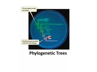
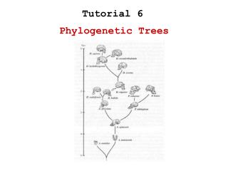
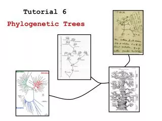
Background • Phylogenetic tree: diagram showing evolutionary lineages of species/genes • Trees are used: • To understand lineage of various species • To understand how various functions evolved • To inform multiple alignments Building phylogenetic trees
Phylogenetic tree approaches • Distance: • UPGMA • Neighbour-joining • Parsimony: • Traditional parsimony • Weighted parsimony Building phylogenetic trees
Making a tree from pairwise distances • Given a set of sequences you want to build a tree. • Compute the distances dijbetween each pair i, j of the sequences. • There are many different distance measures. • Average distance between pairs of sequences from each cluster. Building phylogenetic trees
UPGMA • Unweighted Pair Group Method using arithmetic Averages. • It works by clustering the sequences, at each stage combining two clusters and at the same time creating a new node in a tree, using a distance measure. Building phylogenetic trees
Distance between points • |Ci| and |Cj| denote the number of sequences in clusters i and j. l 3 j 4 2 i Building phylogenetic trees
Distance between clusters • Let Ckbe the union of clusters Ci and Cj,then dkl • Where Cl is any other cluster. l 3 j 4 k i Building phylogenetic trees
Building the tree: UPGMA Initialisation: Assign each sequence i to its own cluster Ci, Define one leaf of T for each sequence, and place at height zero. Iteration: Determine the two clusters i, j for which dij is minimal. Define a new cluster k by , and define dkl for all l. Define a node k with daughter nodes i an j, and place it at height dij /2. Add k to the current clusters and remove i and j. Terminiation: When only two clusters i, j remain, place the root at height dij /2. Building phylogenetic trees
UPGMA: Initialisation Building phylogenetic trees
UPGMA: Iteration 1 Building phylogenetic trees
UPGMA: Iteration 2 Building phylogenetic trees
UPGMA: Iteration 3 Building phylogenetic trees
UPGMA: Terminiation Building phylogenetic trees
Properties of UPGMA • Molecular clock & ultrametric property of distances • Additivity Building phylogenetic trees
Properties of UPGMA:Molecular clock & ultrametric • The molecular clock assumption: divergence of sequences is assumed to occur at the same rate at all points in the tree. • If this does holds, then the data is said to be ultrametric. Building phylogenetic trees
Properties of UPGMA:Additivity • Given a tree, its edge lengths are said to be additive if the distance between any pair of leaves is the sum of the lengths of the edges on the path connecting them. m i k j Building phylogenetic trees
Neighbour-joining • N-j constructs a tree by iteratively joining subtrees (like UPGMA). • Produces an unrooted tree. • Doesn’t make the molecular clock assumption, therefore the ultrametric property does not hold. Building phylogenetic trees
Distances in Neighbour-joining • Given a new internal nodek, the distance to another node m is given by: m i k j Building phylogenetic trees
Distances in Neighbour-joining • Generalizing this so that the distance to all other leaves are taken into account: • Where • And |L| denotes the size of the set L of leaves. m i k j Building phylogenetic trees
Building the tree:Neighbour-joining Initialisation: Define T to be the set of leaf nodes, one for each given sequence, and put L=T. Iteration: Pick a pair i, j in L for which defined by is minimal. Define a new node k and set , for all m in L. Add k to T with edges of lengths , joining k to i and j, respectively. Remove i and j from L and add k. Termination: When L consists of two leaves i and j add the remaining edge between i and j, with length dij. Building phylogenetic trees
outgroup Candidateroot Rooting trees m • Finding a root in an unrooted tree is sometimes accomplished by using an outgroup: • A species known to be more distantly related to remaining species than they are to each other • The point where the outgroup joins the rest of the tree is the best candidate for root position i k l j Building phylogenetic trees
Comments on distance based methods • If the given data is ultrametric (and these distances represent real distances), then UPGMA will identify the correct tree. • If the data is additive (and these distances represent real distances), then Neighbour-joining will identify the correct tree. • Otherwise, the methods may not recover the correct tree, but they may still be reasonable heuristics. Building phylogenetic trees
Phylogenetic tree approaches • Distance: • UPGMA • Neighbour-joining • Parsimony: • Traditional parsimony • Weighted parsimony Building phylogenetic trees
Parsimony • Most widely used tree building algorithm(?). • Finds the tree that explains the data with a minimal number of changes. • Instead of building atree, it assigns a cost to a given tree. • Two components of the parsimony algorithm can be distinguished: • The computation of a cost for a given tree; • A search through all trees, to find the overall minimum of this cost. Building phylogenetic trees
Parsimony example • Given the following sequences: AAG,AAA,GGA,AGA. • Several trees could explain the phylogeny Building phylogenetic trees
Traditional Parsimony • Count the number of substitutions • At each node keep: • a list of minimal cost residues • the current cost • Post-order traversal of the tree Building phylogenetic trees
Traditional Parsimony Initialisation: Set current cost C=0 and k =2n-1, the number of the root node. Recursion: To obtain the set Rk: If k is a leaf node: Set If k is not a leaf node: Compute Ri , Rj for the daughter i, j of k, and set if this intersection is not empty, or else set and increment C. Termination: Minimal cost of tree = C. Building phylogenetic trees
Weighted Parsimony • Extension of the traditional parsimony. • Adds a cost function S(a,b) for each substitution of a by b. • Post-order traversal of the tree • Aim is now to minimize the cost. Building phylogenetic trees
Weighted Parsimony Initialisation: Set k =2n-1, the number of the root node Recursion: Compute Sk(a) for all a as follows: If k is a leaf node: Set , otherwise If k is not a leaf node: Compute Si(a), Sj(a) for all a at the daughter i, j and define Termination: Minimal cost of tree = minaS2n-1(a). Building phylogenetic trees
Break • Questions so far? • After the break: • Assessing the trees: the bootstrap; • Simultaneous alignment and phylogeny; • Application: Phylip Building phylogenetic trees
Branch and bound • Parsimony itself can not build a tree! • Using simple enumeration methods the number of trees become very large very fast. • How to build the trees? • Stochastically • Branch and bound Building phylogenetic trees
Branch and bound • B&B uses the parsimony algorithm. • It guarantees to find the overall best tree. • It systematically builds trees by increasing the number of leaves. • Abandons a particular avenue of tree building whenever the current incomplete tree (T*) has a cost(T*)>cost(Tmin). Building phylogenetic trees
The Bootstrap • A measure how much a tree should be trusted. • Use the bootstrap as a method of assessing the significance of some phylogenetic feature. Building phylogenetic trees
The Bootstrap (2) • The bootstrap works as follows: • Given a dataset of an alignment of sequences. • Generate an artificial dataset of the same size as the original dataset by picking columns from the alignment at random with replacement. • Apply the tree building algorithm to this artificial dataset. • Repeat selection and tree building procedure n times. • The feature with which a chosen phylogenetic features appears is taken to be a measure of the confidence we can have in this feature. Building phylogenetic trees
Simultaneous alignment and phylogeny • Simultaneously aligning sequences and finding a plausible phylogeny: • Sankoff & Cedergren’s gap-substitution algorithm; • Hein’s affine cost algorithm. • Both find an optimal alignment given a tree. Building phylogenetic trees
Sankoff & Cedergren’s gap-substitution algorithm • Guarantees to find ancestral sequences, and alignments of them and the leaf sequences. • It uses a character-substitution model of gaps • Together this minimizes a tree-based parsimony-type cost. • The algorithm is a combination of two known methods: • Dynamic programming method (Chapter 6); • Weighted Parsimony algorithm. Building phylogenetic trees
Hein’s affine cost algorithm • It uses affine gap penalties. • Faster than the Sankoff & Cedergren algorithm. • The aim is to find sequences z at a given node aligned to both of the sequences x and y at the daughter nodes satisfying: • Where S is the total cost for a given alignment of two sequences. (mismatch cost =1 and 0 otherwise) Building phylogenetic trees
Hein’s affine cost algorithm • Compared to equation (2.16) (alignment with affine gap scores) here the algorithm searches for the minimal cost path. • The affine gap cost for a gap of length k isd+(k-1)e, where e<=d. Building phylogenetic trees
VM VX VY Dynamic programming matrix for two sequences i j d=2 e=1 Building phylogenetic trees
Hein’s affine cost algorithm • Find the zfor which is minimal. • From the matrix follows: • C - - A C - • C A C - - - • CAC could be possible z. CAC(?) CAC CTCACA Building phylogenetic trees
Which zcould serve best as ancestor? Hein’s affine cost algorithm CAC(?) CACACA(?) CAC CTCACA CAC CTCACA CACAC(?) CAC CTCACA Building phylogenetic trees
Hein’s affine cost algorithm CAC CACACA CACAC Building phylogenetic trees
Sequence graph • Follow a path through the dynamic programming matrix. • Derive a graph from this matrix. • Whenever a cell is used by an optimal path a vertex is added to the graph. Building phylogenetic trees
Graph 1 Sequence graph Building phylogenetic trees
Graph 2 Sequence graph:line arrangement Graph 1 Building phylogenetic trees
Graph 3 Sequence graph:replacing the dummy edges Graph 2 Building phylogenetic trees
Dynamic Programming matrix:TAC – Graph 3 Building phylogenetic trees
Ancestors • Possible ancestral sequences for the leaf sequences TAC, CAC and CTCACA given the tree shown. • Derived from the sequence graphs. CAC 1 CAC TAC 5 CAC CTCACA Building phylogenetic trees
Limitations of Hein’s model • Hein’s algorithm takes the minimal cost sequences at each node upward. • This can fail to give the overall optimum. • Suppose the cost for a gap of length k is: • 13+3(k-1) • Mismatch: • 4 • Suppose the leaves G and GTT. Building phylogenetic trees