Download
1 / 29
300 likes | 475 Views
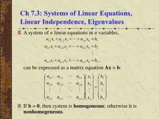
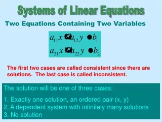
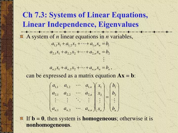
Ch 7.3: Systems of Linear Equations, Linear Independence, Eigenvalues. A system of n linear equations in n variables, can be expressed as a matrix equation Ax = b : If b = 0 , then system is homogeneous ; otherwise it is nonhomogeneous. Nonsingular Case.

E N D
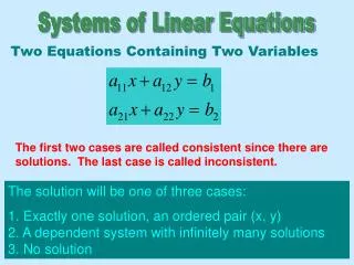
Ch 7.3: Systems of Linear Equations, Linear Independence, Eigenvalues • A system of n linear equations in n variables, can be expressed as a matrix equation Ax = b: • If b = 0, then system is homogeneous; otherwise it is nonhomogeneous.
Nonsingular Case • If the coefficient matrix A is nonsingular, then it is invertible and we can solve Ax = b as follows: • This solution is therefore unique. Also, if b = 0, it follows that the unique solution to Ax = 0 is x = A-10 = 0. • Thus if A is nonsingular, then the only solution to Ax = 0 is the trivial solution x = 0.
Example 1: Nonsingular Case (1 of 3) • From a previous example, we know that the matrix A below is nonsingular with inverse as given. • Using the definition of matrix multiplication, it follows that the only solution of Ax = 0 is x = 0:
Example 1: Nonsingular Case (2 of 3) • Now let’s solve the nonhomogeneous linear system Ax = b below using A-1: • This system of equations can be written as Ax = b, where • Then
Example 1: Nonsingular Case (3 of 3) • Alternatively, we could solve the nonhomogeneous linear system Ax = b below using row reduction. • To do so, form the augmented matrix (A|b) and reduce, using elementary row operations.
Singular Case • If the coefficient matrix A is singular, then A-1 does not exist, and either a solution to Ax = b does not exist, or there is more than one solution (not unique). • Further, the homogeneous system Ax = 0 has more than one solution. That is, in addition to the trivial solution x = 0, thereare infinitely many nontrivial solutions. • The nonhomogeneous case Ax = b has no solution unless (b, y) = 0, for all vectors y satisfying A*y = 0, where A* is the adjoint of A. • In this case, Ax = b has solutions (infinitely many), each of the form x = x(0) + , where x(0) is a particular solution of Ax = b, and is any solution of Ax = 0.
Example 2: Singular Case (1 of 3) • Solve the nonhomogeneous linear system Ax = b below using row reduction. • To do so, form the augmented matrix (A|b) and reduce, using elementary row operations.
Example 2: Singular Case (2 of 3) • Solve the nonhomogeneous linear system Ax = b below using row reduction. • Reduce the augmented matrix (A|b) as follows:
Example 2: Singular Case (3 of 3) • From the previous slide, we require • Suppose • Then the reduced augmented matrix (A|b) becomes:
Linear Dependence and Independence • A set of vectors x(1), x(2),…, x(n) is linearly dependent if there exists scalars c1, c2,…, cn, not all zero, such that • If the only solution of is c1= c2 = …= cn = 0, then x(1), x(2),…, x(n) is linearly independent.
Example 3: Linear Independence (1 of 2) • Determine whether the following vectors are linear dependent or linearly independent. • We need to solve or
Example 3: Linear Independence (2 of 2) • We thus reduce the augmented matrix (A|b), as before. • Thus the only solution is c1= c2 = …= cn = 0, and therefore the original vectors are linearly independent.
Example 4: Linear Dependence (1 of 2) • Determine whether the following vectors are linear dependent or linearly independent. • We need to solve or
Example 4: Linear Dependence (2 of 2) • We thus reduce the augmented matrix (A|b), as before. • Thus the original vectors are linearly dependent, with
Linear Independence and Invertibility • Consider the previous two examples: • The first matrix was known to be nonsingular, and its column vectors were linearly independent. • The second matrix was known to be singular, and its column vectors were linearly dependent. • This is true in general: the columns (or rows) of A are linearly independent iff A is nonsingular iff A-1 exists. • Also, A is nonsingular iff detA 0, hence columns (or rows) of A are linearly independent iff detA 0. • Further, if A = BC, then det(C) = det(A)det(B). Thus if the columns (or rows) of A and B are linearly independent, then the columns (or rows) of C are also.
Linear Dependence & Vector Functions • Now consider vector functions x(1)(t), x(2)(t),…, x(n)(t), where • As before, x(1)(t), x(2)(t),…, x(n)(t) is linearly dependent on I if there exists scalars c1, c2,…, cn, not all zero, such that • Otherwise x(1)(t), x(2)(t),…, x(n)(t) is linearly independent on I See text for more discussion on this.
Eigenvalues and Eigenvectors • The eqn. Ax = y can be viewed as a linear transformation that maps (or transforms) x into a new vector y. • Nonzero vectors x that transform into multiples of themselves are important in many applications. • Thus we solve Ax = x or equivalently, (A-I)x = 0. • This equation has a nonzero solution if we choose such that det(A-I) = 0. • Such values of are called eigenvalues of A, and the nonzero solutions x are called eigenvectors.
Example 5: Eigenvalues (1 of 3) • Find the eigenvalues and eigenvectors of the matrix A. • Solution: Choose such that det(A-I) = 0, as follows.
Example 5: First Eigenvector (2 of 3) • To find the eigenvectors of the matrix A, we need to solve (A-I)x = 0 for = 3 and = -7. • Eigenvector for = 3: Solve by row reducing the augmented matrix:
Example 5: Second Eigenvector (3 of 3) • Eigenvector for = -7: Solve by row reducing the augmented matrix:
Normalized Eigenvectors • From the previous example, we see that eigenvectors are determined up to a nonzero multiplicative constant. • If this constant is specified in some particular way, then the eigenvector is said to be normalized. • For example, eigenvectors are sometimes normalized by choosing the constant so that ||x|| = (x, x)½ = 1.
Algebraic and Geometric Multiplicity • In finding the eigenvalues of an n x n matrix A, we solve det(A-I) = 0. • Since this involves finding the determinant of an n x n matrix, the problem reduces to finding roots of an nth degree polynomial. • Denote these roots, or eigenvalues, by 1, 2, …, n. • If an eigenvalue is repeated m times, then its algebraic multiplicity is m. • Each eigenvalue has at least one eigenvector, and a eigenvalue of algebraic multiplicity m may have q linearly independent eigevectors, 1 q m, and q is called the geometric multiplicity of the eigenvalue.
Eigenvectors and Linear Independence • If an eigenvalue has algebraic multiplicity 1, then it is said to be simple, and the geometric multiplicity is 1 also. • If each eigenvalue of an n x n matrix A is simple, then A has n distinct eigenvalues. It can be shown that the n eigenvectors corresponding to these eigenvalues are linearly independent. • If an eigenvalue has one or more repeated eigenvalues, then there may be fewer than n linearly independent eigenvectors since for each repeated eigenvalue, we may have q < m. This may lead to complications in solving systems of differential equations.
Example 6: Eigenvalues (1 of 5) • Find the eigenvalues and eigenvectors of the matrix A. • Solution: Choose such that det(A-I) = 0, as follows.
Example 6: First Eigenvector (2 of 5) • Eigenvector for = 2: Solve (A-I)x = 0, as follows.
Example 6: 2nd and 3rd Eigenvectors (3 of 5) • Eigenvector for = -1: Solve (A-I)x = 0, as follows.
Example 6: Eigenvectors of A(4 of 5) • Thus three eigenvectors of A are where x(2), x(3) correspond to the double eigenvalue = - 1. • It can be shown that x(1), x(2), x(3)arelinearly independent. • Hence A is a 3 x 3 symmetric matrix (A = AT ) with 3 real eigenvalues and 3 linearly independent eigenvectors.
Example 6: Eigenvectors of A(5 of 5) • Note that we could have we had chosen • Then the eigenvectors are orthogonal, since • Thus A is a 3 x 3 symmetric matrix with 3 real eigenvalues and 3 linearly independent orthogonal eigenvectors.
Hermitian Matrices • A self-adjoint, or Hermitian matrix, satisfies A = A*, where we recall that A* = AT . • Thus for a Hermitian matrix, aij = aji. • Note that if A has real entries and is symmetric (see last example), then A is Hermitian. • An n x n Hermitian matrix A has the following properties: • All eigenvalues of A are real. • There exists a full set of n linearly independent eigenvectors of A. • If x(1) and x(2)are eigenvectors that correspond to different eigenvalues of A, then x(1) and x(2)are orthogonal. • Corresponding to an eigenvalue of algebraic multiplicity m, it is possible to choose m mutually orthogonal eigenvectors, and hence A has a full set of n linearly independent orthogonal eigenvectors.