An Introduction to R

1. An Introduction to R 96325125 鐘英愷 93316150 劉郁彧 93316105 梁詩屏 93316113 陳泓君

2. Outline • The R environment • R and Statistics • Data Import/export • Basic Operator • Programming in R • Graphics

3. The R environment R is an integrated suite of software facilities for data manipulation, calculation and graphical display. Among other things it has : • an effective data handling and storage facility, • a suite of operators for calculations on arrays, in particular matrices, • a large, coherent, integrated collection of intermediate tools for data analysis, graphical facilities for data analysis and display either directly at the computer or on hard-copy, and • a well developed, simple and effective programming language (called `S') which includes conditionals, loops, user defined recursive functions and input and output facilities. (Indeed most of the system supplied functions are themselves written in the S language.)

4. The term “environment" is intended to characterize it as a fully planned and coherent system, rather than an incremental accretion of very specific and inflexible tools, as is frequently the case with other data analysis software. • R is a newly developing methods of interactive data analysis. It has developed rapidly, and has been extended by a large collection of packages.

5. R with Statistics? • R is a system for statistical analyses and graphics created by Ross Ihaka and Robert Gentleman. • R is both a software and a language considered as a dialect of the language S created by the AT&T Bell Laboratories. S is available as the software S-PLUS commercialized by Insightful.

6. How it make& where we get it • R is available in several forms: the sources written mainly in C (and some routines in Fortran), essentially for Unix and Linux machines, or some pre-compiled binaries for Windows, Linux (Debian, Mandrake, RedHat, SuSe), Macintosh and Alpha Unix. • The files needed to install R, either from the sources or from the pre-compiled binaries, are distributed from the internet site of the Comprehensive R Archive Network(CRAN) where the instructions for the installation are also available. http://CRAN.R-project.org

8. R has many functions for statistical analyses and graphics; the latter are visualized immediately in their own window and can be saved in various formats (jpg, png, bmp, ps, pdf, emf, pictex, xfig). • The results from a statistical analysis are displayed on the screen, some intermediate results (P-values, regression coefficients, residuals, . . . ) can be saved, written in a file, or used in subsequent analyses.

9. There is an important difference between S (and hence R) and the other main statistical systems. • In S a statistical analysis is normally done as a series of steps, with intermediate results being stored in objects. • SAS and SPSS will give copious output from a regression or discriminant analysis, R will give minimal output and store the results in a t object for subsequent interrogation by further R functions.

10. Disadvantages of R • R is not efficient in handling large data sets. • Slow computation for a large number of do-loops, compared to C/C++, Fortran etc. • Self-Learning is not so convenient compared to “point-and-click” statistics software. • No warrantee and informal support. • Needed to upgrade R version to install some newly developed packages.

11. Getting Help in R • library()#lists all available libraries on system • help(command)#getting help for one command, e.g. help(heatmap) • help.search(“topic”)#searches help system for packages associated with the topic, e.g. help.search(“distribution”) • help.start()#starts local HTML interface • q()#quits R console

12. Basic Usage of R • The general R command syntax uses the assignment operator “<-”(or “=“) to assign data to object. • object <- function (arguments) • source(“myscript.R”), #command to execute an R script named as myscript.R. • objects()or ls(), # list the names of all objects • rm(data1), #Remove the object named data1 from the current environment • data1 <-edit(data.frame())# Starts empty GUI spreadsheet editor for manual data entry.

13. Basic Usage of R • class(object)#displays the object type. • str(object)#displays the internal type and structure of an R object. >str(m) num [1:4, 1:3] 0.248 0.589 -0.589 0.504 1.524 ... • attributes(object)#Returns an object's attribute list. > attributes(m) $dim [1] 4 3 • dir()# Reads content of current working directory. • getwd()# Returns current working directory. • setwd("/home/user")# Changes current working directory to user specified directory.

14. Data Import • read.delim("clipboard", header=T)# Command to copy&pastetables from Excel or other programs into R. If the 'header' argument isset to FALSE, then the first line of the data set will not be used as column titles. • scan("my_file")# reads vector/array into vector from file or keyboard. • my_frame<-read.delim(“c://Affymetrix/affy1.txt", na.strings= "", fill=TRUE, header=T, sep="\t")# The function read.delim() is often more flexible for importing tables with empty fields and long character strings (e.g. gene descriptions). • It supports data import on the web. • Different coding of missing values (na.strings=“NA”or “”). Data columns can be separated by TAB, comma, or semicolon (sep=“”).

15. Data Import There are some alternatives for reading data as followings. • my_frame<-read.table(file=“path", header=TRUE, sep="\t")#Reads in table with info on column headers and field separators. data<-read.table("http://www.cmu.edu.tw/example.txt", header=TRUE) • my_frame<-read.csv(file=“path“, header=TRUE)# reads .csvfile with comma separated value. • You can skip lines, read a limited number of lines, different decimal separator, and more importing options. • The foreign package can read files from Stata, SAS, and SPSS.

16. Data Export • write.table(iris, "clipboard", sep="\t", col.names=NA, quote=F)# Command to copy&pastefrom R into Excel or other programs. It writes the data of an R data frame object into the clipbroardfrom where it can be pasted into other applications. • write.table(dataframe, file=“file path", sep="\t", col.names= NA)# Writes data frame to a tab-delimited text file. The argument 'col.names= NA' makes sure that the titles align with columns when row/index names are exported (default). • write(x, file="file path")# Writes matrix data to a file.

17. Basic Operators • Comparison operators • equal: == • not equal: != • greater/less than: > / < • greater/less than or equal: >= <= Example: 1 == 1# Returns TRUE. • 􀂆Logical operators • AND:& x <- 1:10; y <- 10:1 # Creates the sample vectors 'x' and 'y'. x > y & x > 5 # Returns TRUE where both comparisons return TRUE. • OR: | x == y | x != y # Returns TRUE where at least one comparison returns TRUE. • NOT: ! !x > y # The '!' sign returns the negation (opposite) of a logical vector.

18. Basic Operators • Calculations • Four basic arithmetic functions: addition, subtraction, multiplication and division 1 + 1; 1 - 1; 1 * 1; 1 / 1 # Returns the results of these calculations. • Calculations on vectors x <- 1:20; sum(x); mean(x), sd(x); sqrt(x) ;rank(x);sort(x) # Calculates for the vector x its sum, mean, standard deviation and square root etc. x <- 1:20; y <- 1:20; x + y # Calculates the sum for each element in the vectors x and y.

19. Data Types • Numeric data: 1, 2, 3 x <- c(1, 2, 3); x; is.numeric(x); as.character(x) # Creates a numeric vector, checks for the data type and converts it into a character vector. • Character data: "a", "b" , "c" x <- c("1", "2", "3"); x; is.character(x); as.numeric(x) #Creates a character vector, checks for the data type and converts it into a numeric vector. • Logical data: TRUE, FALSE, TRUE 1:10 < 5 # Returns TRUE where x is < 5.

20. Object Types • vectors: ordered collection of numeric, character, complex and logical values. • factors: special type vectors with grouping information of its components • data frames: two dimensional structures with different data types • matrices: two dimensional structures with data of same type • arrays: multidimensional arrays of vectors • lists: general form of vectors with different types of elements • functions: piece of code

21. Subsetting Syntax • my_object[index]# Subsettingof one dimensional objects, like vectors and factors. Returns elements with positions in index • my_object[row.index, col.index]# Subsettingof two dimensional objects, like matrices and data frames. • my_object[row.index, col.index, dim]# Subsettingof three dimensional objects, like arrays. • dim(my_object)# Returns the numbers of row and column • my_logical<-(my_object> 10)# Generates a logical vector as example. • my_object[my_logical] # Returns the elements where my_logical contains TRUE values. • my_object$Name1 # Returns the ‘Name1' column in the my_objectdata frame.

22. Vector & List • vector: an ordered collection of data of the same type. • > a = c(7,5,1) • > a[2] • [1] 5 • list: an ordered collection of data of arbitrary types. > doe = list(name="john",age=28,married=F) • > doe$name • [1] "john“ • > doe$age • [1] 28 • Typically, vector elements are accessed by their index (an integer), list elements by their name (a character string). But both types support both access methods.

23. Programming in R • Ifelse Statement: Example : x <- 1:10 ifelse(x<5 | x>8, x, 0) • For Loop : Example: mean mydf <- iris myve <- NULL for(i in 1:length(mydf[,1])) { myve <- c(myve, mean(as.vector(as.matrix(mydf[i,1:3])))) }

24. While Loop: Example z <- 0 while(z<5) { z <- z+2 print(z) } • Writing your own functions > f=function(x){x^2+2*x} >f(3) [1] 15

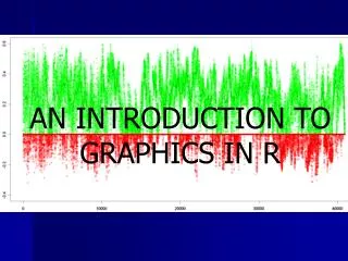
25. Graphics library(UsingR) scatter.with.hist(faithful$eruptions,faithf ul$waiting)

26. Reference • 2007年 R統計軟體研習會-------蔡政安 教授 http://www.statedu.ntu.edu.tw/2007conference/index.htm • An Introduction to R http://cran.r-project.org/doc/manuals/R-intro.pdf

27. ~The End~ Thanks for your listening.