Human vs. Machine

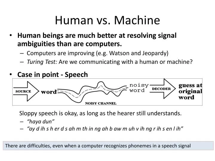
1. Human vs. Machine • Human beings are much better at resolving signal ambiguities than are computers. • Computers are improving (e.g. Watson and Jeopardy) • Turing Test: Are we communicating with a human or machine? • Case in point - SpeechSloppy speech is okay, as long as the hearer still understands. • “haya dun” • “ay d ih s h er d s ah m th in ng ah b aw m uh v ihng r ih s en l ih” There are difficulties, even when a computer recognizes phonemes in a speech signal

2. One sentence, eight possible meanings I made her duck • I cooked waterfowl for her. • I stole her waterfowl and cooked it. • I used my abilities to create a living waterfowl for her. • I caused her to bid low in the game of bridge. • I created the plastic duck that she owns. • I caused her to quickly lower her head or body. • I waved my magic wand and turned her into waterfowl. • I caused her to avoid the test.

3. Robot-human dialog 99% accuracy Robot: “Hi, my name is Robo. I am looking for work to raise funds for Natural Language Processing research.” Person: “Do you know how to paint?” Robo: “I have successfully completed training in this skill.” Person: “Great! The porch needs painting. Here are the brushes and paint.” Robot rolls away efficiently. An hour later he returns. Robo: “The task is complete.” Person: “That was fast, here is your salary; good job, and come back again.” Robo speaks while rolling away with the payment. Robo: “The car was not a Porche; it was a Mercedes.” Moral: You need a sense of humor to work in this field.

4. Challenges Speaker variability Slurring and running words together Co-articulation Handling words not in the vocabulary Grammar Complexities Speech semantics Recognizing idioms Background noise Signal transmission distortion Approaches Use large pre-recorded data samples Train for particular users Require artificial pauses between words Limit vocabulary size Limit the grammar Use high quality microphones Require low noise environments Difficulties Today's best systems cannot match human perception

5. ASR Difficulties • Realizations are points in continuous space, not discrete • Sounds take characteristics of adjacent sounds (assimilation) • Sounds that are combinations of two (co-articulation) • Articulator targets are often not reached • Diphthongs combine different phonemes • Adding (epenthesis) or deleting (elision) • Missing word, phrase boundaries, endings • Many tonal variations during speech • Varied vowel durations • Common knowledge, familiar background leads to more sloppy speech with additional non-linearities.

6. Possible Applications • Compare two audio signals to compare speaker’s utterance to records from a database of recordings • Convert audio into a text document • Visually represent the vocal tract of the speaker in real time • Recognize a particular speaker for enhanced security • Transform audio signal to enhance its speech qualities • Perform tasks based on user commands • Recognize the language and perform appropriately

7. A sample of issues to consider • Can we assume the target language or is the application to be language independent? • Is there access to databases describing grammatical, morphological, and phonological rules? • Are there digital dictionaries available? Does the application require a large dictionary? • Are there corpora available to scientifically measure performance against other implementations? • How does the system perform when the SNR is low? What is a typical SNR characteristics when the application is in use? • What is the accuracy requirements for the application? • Are statistical training procedures practical for the application?

8. Phonological Grammars Phonology: Study of sound combinations • Sound Patterns • English: 13 features for 8192 combinations • Complete descriptive grammar • Rule based, meaning a formal grammar can represent valid sound combinations in a language • Unfortunately, these rules are language-specific • Recent research • Trend towards context-sensitive descriptions • Little thought concerning computational feasibility • Listeners likely don’t perceive using thousands of rules

9. Formal Grammars (Chomsky 1950) • Formal grammar definition: G = (N, T, s0, P, F) • N is a set of non-terminal symbols (or states) • T is the set of terminal symbols (N ∩ T = {}) • S0a start symbol • P is a set of production rules • F (a subset of N) is a set of final symbols • Right regular grammar productions have the forms B → a, B → aC, or B → "" where B,C∈N and a∈ T • Context Free (Programming language) productions have forms B → w where B ∈ N and w is a possibly empty string from N, T • Context Sensitive (Natural language) productions have forms αAβ → αγβ or αAβ  ""where A∈N and α,γ,β∈(N U T)* abd |αAβ|≤|αγβ|

10. Chomsky Language Hierarchy

11. Classifying the Chomsky Grammars • Notes • Regular • Left hand side contains one non terminal, right hand has only one non-terminal • Context Free • Left hand side contains one non-terminal, right hand side mixes terminals and non-terminals • Context sensitive • Left hand side has both terminals and non-terminals • Turing Equivalent: All rules are fair game (computational power of a computer)

12. Context Free Grammars Chomsky (1956) Backus (1959) • Capture constituents and ordering • Regular grammars are too limited to represent grammars • Context Free Grammars consist of • Set of non-terminal symbols N • Finite alphabet of terminals  • Set of productions A → such that AN, -string  (N)* • A designated start symbol • Used for programming language syntax. Too restrictive for natural languages

13. Example Grammar (L0)

14. Context Free Grammars for Natural Language • Context free grammars work well for basic grammar syntax • Disadvantage • Some complex syntactical rules requires clumsy constructions • Agreement: He ate many meal • Movement of grammatical components: • Which flight do you want me to have the travel agent book? • The object is far from its matching verb

15. Morphology • How phonemes combine to make words • Important for speech recognition and synthesis • Example: singular to plural • Run to runs: z sound (voiced) • Hit to Hits: s sound (unvoiced) • One approach: Devise language specific sets of rules of pronunciation

16. Syllables • Organizational phonological unit • Vowel between two consonants • Ambiguous positioning of consonants into syllables • Tree structured representation • Basic unit of prosody • Lexical stress: inherent property of a word • Sentential stress: speaker choice to emphasize or clarrify

17. Finite State Automata • Definition: (N, T, s0, δ, F) where • N is a finite, non-empty set of non-terminal states • T is a finite, non-empty set of terminal symbols • s0 is an initial state, an element of • δ is the state-transition function • Deterministic transition function: δ :Sx∑S • Nondeterministic transition function: δ:Sx∑P⊂S • Transducers: add Γ, a set of output symbols and ω:ΓO • F⊂S is the (possibly empty) set of final states

18. Finite-state Automata Equivalent to: • Finite-state automata (FSA) • Regular languages • Regular expressions

19. baa! baaa! baaaa! baaaaa! ... /baa+!/ a b a a ! q0 q1 q2 q3 q4 finalstate state transition Finite-state Automata (Machines)

20. q0 a b a ! b a b a a ! 0 1 2 3 4 Input Tape REJECT

21. q4 q0 q1 q2 q3 q3 a b a a a b a a ! ! 0 1 2 3 4 Input Tape ACCEPT

22. State-transition Tables

23. Finite State Machine Examples Deterministic Non deterministic

24. Finite State Transducer A Finite State Automata that produces an output string Input: Features from a sequence of frames Processing: Find the most likely path through the sequence using hidden Markov models or Neural Networks Output: The most likely word, phoneme, or syllable O is a set of output states, ω: S->O

25. Back End Processing • Rule Based: Insufficient to represent the differences in how words are constructed • Statistics based: Most other areas of Natural Language processing are trending to statistical-based methods • Procedure • Supervised training: An algorithm “learns” the parameters using a training set of data. The “trained” algorithm then is ready to run in an actual environment. • Unsupervised training: An algorithm trains itself by computing categories from the training data

26. Representing Stress • There have been unsuccessful attempts to automatically assign stress to phonemes • Notations for representing stress • IPA (International Phonetic Alphabet) has a diacritic symbol for stress • Numeric representation • 0: reduced, 1: normal, 2: stressed • Relative • Reduced (R) or Stressed (S) • No notation means undistinguished

27. Random Variables • Random Variable, X, is a quantity that assigns a numerical value to each possible event • Reason: It would not be possible to analyze the results without this. • Example: pick a ball out of a bag. Suppose the balls are red, blue, and green. We could assign X=0 if red, X=1 if blue, and X=2 if green. • Discrete random variable has a finite number of possible values (∑i=1,np(xi) = ∑i=1,nP(X=xi) = 1).

28. Probability Chain Rule • Conditional Probability P(A1,A2) = P(A1) * P(A2|A1) • The Chain Rulegeneralizes to multiple events • P(A1, …,An) = P(A1) P(A2|A1) P(A3|A1,A2)…P(An|A1…An-1) • Examples: • P(the dog) = P(the) P(dog | the) • P(the dog bites) = P(the) P(dog | the) P(bites| the dog) • Conditional probability applies more than individual relative word frequencies because they consider the context • Dog may be relatively rare word in a corpus • But if we see barking, P(dog|barking) is much more likely • In general, the probability of a complete string of words w1…wn is: P(w ) = P(w1)P(w2|w1)P(w3|w1..w2)…P(wn|w1…wn-1) • = • Note: A large n requires a lot of data; chains of two or three work well n 1

29. Probability Density Function • f(x) is a continuous probability density function if ∫-∞, ∞ f(x)dx = 1 a b 0 Note: The shaded area is the probability that a <= x <= b

30. Mean, Variance, Standard Deviation • The mean or expected value • Discrete: µ = E(x) = ∑ x p(x) over all x values • Continuousµ = E(x) = ∫ x f(x) dx from -∞ to∞ • Variance • Discrete: σ2 = ∑(x - µ)2 p(x)= ∑x2p(x) – (∑xp(x))2 • Continuous: σ2 = ∫(x - µ)2f(x)dx = ∫x2dx – (∫xf(x)dx)2 • Standard Deviation: σ = square root of variance • Intuition • Mean: center of the distribution (1st moment) • Variance: spread of the distribution (2nd moment) • standard deviation: percent within a distance from the mean • Skew: asymmetry of the distribution (3rd moment) • Kurtosis: how peaked is the distribution (4th moment)

31. Note: Same mean, different variances

32. Example • Bag of numbered balls • Pick a single ball from the bag • Mean: (µ = ∑ x p(x) ) 1*8/30 + 2*5/30 + 3*3/30 + 4*10/30 + 5*4/30 = 87/30 = 2.9 • Variance Method 1: σ2 = ∑(x - µ)2 p(x) σ2 = 8/30*(-1.9)2 + 5/30*(-0.9)2 + 3/30*0.12 + 10/30*1.12 + 4/30*2.12 = 2.09 • Variance Method 2 (without mean): σ2 = ∑x2p(x)–(∑xp(x))2σ2 = 1*8/30 + 4*5/30 + 9*3/30 + 16*10/30 + 25*4/30 – (1*8/30+2*5/30+3*3/30+4*10/30+5*4/30)2 = 10.5–2.92 = 2.09 • Standard Deviation = (2.09)1/2 ≈ 1.45

33. Covariance Covariance determines how two random variables relate • A positive covariance occurs if two random variables tend to both be above or below their means together • A negative covariance occurs when the random variables tend to be on opposite sides of the mean • If no correlation, the covariance will be close to zero • Covariance formula • Discrete: Cov(X,Y) = ∑x ∑y (x-µx)p(x) * (y-µy)p(y) • Continuous: Cov(X,Y) = ∫x ∫y (x-µx)f(x) * (y-µy)f(y) dy dx • Correlation coefficient: ρxy = Cov(x,y)/(σx*σy) or Cov(x,y)/(N-1) • Numbers greater than unity imply the variables are related

34. Covariance (Dispersion) Matrix • Given Random variables • The covariance matrix ∑, where ∑i,j = E(Xi-ui)(Xj-uj) = cov(xi,xj) • Equivalent Matrix Definition: ∑ = E[(X – E[X])(X – E[X})T] • Note: The T means transpose, some use a single quote instead

35. Covariance Example Three random variables (x0, x1, x2), five observations (N = 5) each Note: ∑ results from the multiplication of the 5x3 matrix and its 3x5 transpose ∑

36. Uniform Distribution The probability of every value is equal • pdf: f(x) = 1 / (b-a) a≤x≤b; 0 otherwise • µ = (a + b)/2, Variance: 1/12 (b-a)2 • Initial training data for acoustic information can be set up as a uniform distribution

37. Binomial Distribution Repeated experiments each with two possible outcomes • pdf: where and n = # of experiments p = success probability • µ = np • σ2 = np(1-p)

38. Multinomial Distribution Number of successes in n independent experiments • pdf: • µi = n pi • σi2 = n pi (1-pi) • Cov(xi,xj) = -npipj • Extends the binomial distribution to multiple random variables

39. Gaussian Distribution • When we analyze probability involving many random processes, the distribution is almost always Gaussian. • Central Limit Theorem: As the sample size of random variables approach ∞, the distribution approaches Gaussian • Probability distribution: f(x | µ,σ2) = 1/(2 πσ)½ *ezwhere z = -(x-µ)2 / (2 σ2)

40. Multivariate Mixture Gaussian Distribution • Multiple independent random variables • Each variable can have its own mean and variance Two independent random variables X and Y

41. Multivariate Normal Distribution

42. Determinant of a 3x3 Matrix Example: Compute Determinant of:

43. B A3 A2 A4 B A1 A5 Bayes' Rule Fundamental to many speech recognition algorithms • P(A | B) = P(B | A)*P(A) P(B) • P(B) =∑k=1,n P(B | Ak) * P(Ak) • P(Ai | B) = P(B|Ai)P(Ai) ∑k=1,n P(B | Ak) * P(Ak) Max [P(word | sound)] = Max [P(sound | word) * P(word) / P(sound)] = Max [P(sound | word) * P(word)] because the denominator is a constant

44. Bayes Example Probability that a car will be late to its destination

45. Noisy Channel Source Decoder Noisy Channel Decoding • Assume Input=word w; Feature vector=f, V=vocabulary • We want to find the word, w = max wεv p(w|f) • Using Bayes Rule: maxwεv p(f|w)p(w)/p(f) • Why use Bayes Rule? • P(w|f) is difficult to compute • P(f|w) is relatively easy to compute. Just add probabilities to reflect spelling or pronunciation variation rules • P(w) is how often w occurs in a large corpus (prior priority) • Ignore P(f). f doesn’t change as we search the lexicon.

46. Bayesian Inference 4 Vegetarians • Randomly choose students from population of ten. Find probabilities: • p(vegetarian) = .4, p(cs major) = .3 • Studentvegetarian is a CS major? p(c|v) = .5 = p(c) p(v|c) / p(v) • Student is a vegetarian andCS major? p(c,v) = .2 = p(v) p(c|v) • Student vegetarianand CS major? p(c,v) = .2 = p(c) p(v|c) • Student CS major is a vegetarian? p(v|c) = .66 = p(v) p(c|v) / p(c) 3 CS majors

47. Definitions • Stochastic process: A process of change of one or random variables {Xi} over time based on a well-defined set of probabilities • Markov model: a Markov model consists of a list of the possible states of that system, the possible transitions from one state to another, and the rates that govern those transitions. Transitions can depend on the current state and some number of previous states. • Markov Chain • Markov model with a finite number of states in which the probability of a next state depends only upon the current state and the immediate past state • Examples • The next phoneme’s probability depends solely on the preceding one of the sequence • A model of word or phoneme prediction that uses the previous N-1 words or phonemes to predict the next (N-gram model) • Hidden Markov model, predicting the hidden cause after observing the output (predicting the words, when observing the features)

48. Vector Quantization • Partition the data into cells (Ci) • Cell centroids quantized as zi • Compute distance between received data and centroids • Received data • quantized into one of the cells • q(x)=ziif x in cell Ciboundary • Distortion (distance) formulas • Euclidian: d(x,z) = ∑i=1,D(xi–zi)2 • Linear: d(x,z) = (x-z)T∑-1 (x-z) • Mahalanobs: Euclidian/ variance • D is the quantization codebook size

49. K- Means Algorithm • Input: • F = {f1, …, fk} is a list of feature vectors • N = desired number of categories (phoneme types) • Output: • C = {c1, …, cN) center of each category • m: F->C Maps feature vector to one of the categories • Pseudocode Randomly put members of F into an initial C WHILE true FOR EACH fj ∈ F assign fj to the closest ck IF no reassignments have taken place THEN BREAK Recompute the center of each member of C • Issues • What is the metric that we use to compute distances? • A poor initial selection will lead to incorrect results or poor performance

50. LBG Extension of K Means Linde, Buzo, and Gray • Let M= 1 to form a single partition • Find centroid of all training data ( 1/T ∑i=0,Txi ) • While (M < desired number of partitions) For each M • Compute centroid position • Replace old centroid with new one • Partition the partition in half • Estimate centroid in each half • Use the k-means algorithm to optimize centroid position • M = 2*M