Download
1 / 1
30 likes | 80 Views
U. Skiba , S. Jones, N. Cowan, D. Famulari, M. Anderson, J. Drewer, Centre for Ecology and Hydrology, Edinburgh, UK D. Chadwick, Rothamsted Research , North Wyke , UK. Rational

E N D
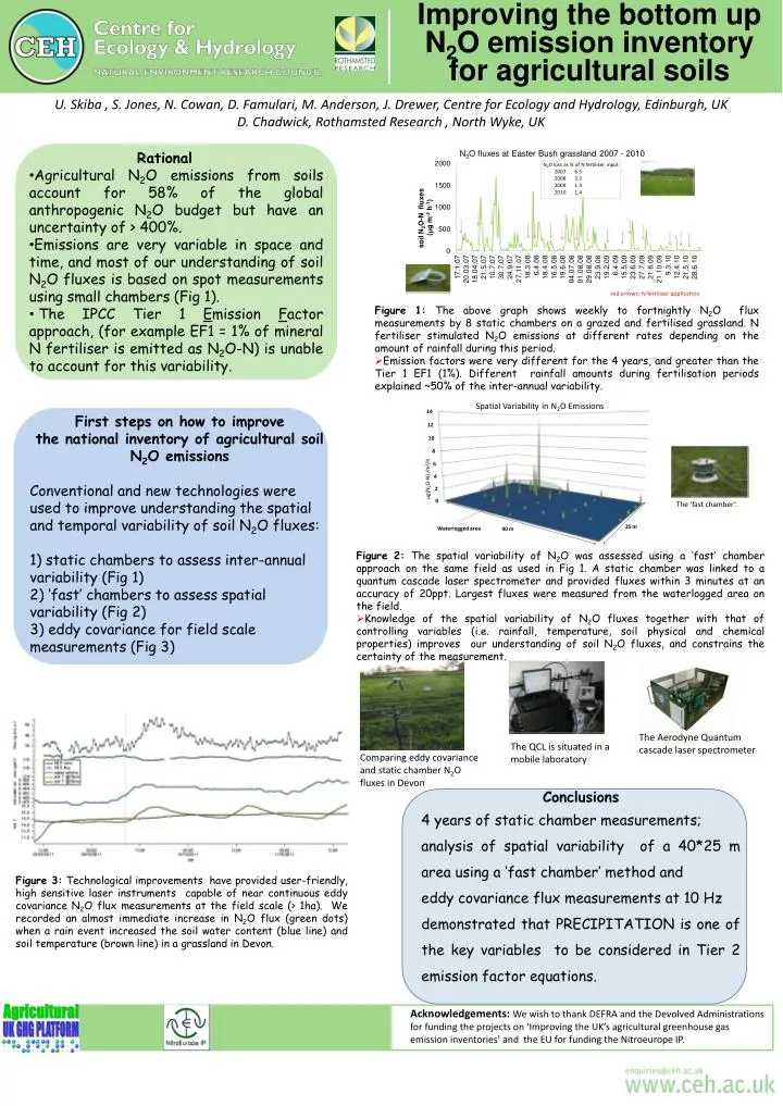
U. Skiba , S. Jones, N. Cowan, D. Famulari, M. Anderson, J. Drewer, Centre for Ecology and Hydrology, Edinburgh, UK D. Chadwick, Rothamsted Research , North Wyke, UK • Rational • Agricultural N2O emissions from soils account for 58% of the global anthropogenic N2O budget but have an uncertainty of > 400%. • Emissions are very variable in space and time, and most of our understanding of soil N2O fluxes is based on spot measurements using small chambers (Fig 1). • The IPCC Tier 1 Emission Factor approach, (for example EF1 = 1% of mineral N fertiliser is emitted as N2O-N) is unable to account for this variability. • Figure 1: The above graph shows weekly to fortnightly N2O flux measurements by 8 static chambers on a grazed and fertilised grassland. N fertiliser stimulated N2O emissions at different rates depending on the amount of rainfall during this period. • Emission factors were very different for the 4 years, and greater than the Tier 1 EF1 (1%). Different rainfall amounts during fertilisation periods explained ~50% of the inter-annual variability. The ‘fast chamber’. • Figure 2: The spatial variability of N2O was assessed using a ‘fast’ chamber approach on the same field as used in Fig 1. A static chamber was linked to a quantum cascade laser spectrometer and provided fluxes within 3 minutes at an accuracy of 20ppt. Largest fluxes were measured from the waterlogged area on the field. • Knowledge of the spatial variability of N2O fluxes together with that of controlling variables (i.e. rainfall, temperature, soil physical and chemical properties) improves our understanding of soil N2O fluxes, and constrains the certainty of the measurement. The Aerodyne Quantum cascade laser spectrometer The QCL is situated in a mobile laboratory Comparing eddy covariance and static chamber N2O fluxes in Devon Conclusions 4 years of static chamber measurements; analysis of spatial variability of a 40*25 m area using a ‘fast chamber’ method and eddy covariance flux measurements at 10 Hz demonstrated that PRECIPITATION is one of the key variables to be considered in Tier 2 emission factor equations. Figure 3: Technological improvements have provided user-friendly, high sensitive laser instruments capable of near continuous eddy covariance N2O flux measurements at the field scale (> 1ha). We recorded an almost immediate increase in N2O flux (green dots) when a rain event increased the soil water content (blue line) and soil temperature (brown line) in a grassland in Devon. Improving the bottom up N2O emission inventory for agricultural soils Acknowledgements: We wish to thank DEFRA and the Devolved Administrations for funding the projects on ‘Improving the UK’s agricultural greenhouse gas emission inventories’ and the EU for funding the Nitroeurope IP. First steps on how to improve the national inventory of agricultural soil N2O emissions Conventional and new technologies were used to improve understanding the spatial and temporal variability of soil N2O fluxes: 1) static chambers to assess inter-annual variability (Fig 1) 2) ‘fast’ chambers to assess spatial variability (Fig 2) 3) eddy covariance for field scale measurements (Fig 3)