Download
1 / 26
260 likes | 354 Views
Objective : To estimate population means with various confidence levels. Chapter 6 6.1-6.4: Estimating a Population Mean. Descriptive Statistics – a summary or description of data (usually the calculation)

E N D
Objective: To estimate population means with various confidence levels Chapter 66.1-6.4: Estimating a Population Mean
Descriptive Statistics – a summary or description of data (usually the calculation) • Ex) The mean grade for Ms. Halliday’s CHS Statistics students on the 5.1 – 5.4 Quiz was 89.1. (89.1 is the descriptive statistic) • Inferential Statistics – when we use sample data to make generalizations (inferences) about a population • We use sample data to: • Estimate the value of a population parameter • Test the claim (or hypothesis) about a population • Chapter 6 is dedicated to presenting the methods for determining inferential statistics. 6.1 - Review
Here is a list of 99 body temperatures obtained by the University of Maryland. Calculate the descriptive statistics for these data (mean, standard deviation, sample size). Discuss the shape, center, and spread, as well as any outliers. 98.6 98.6 98.0 98.0 99.0 98.4 98.4 98.4 98.4 98.6 98.6 98.8 98.6 97.0 97.0 98.8 97.6 97.7 98.8 97.6 97.7 98.8 98.0 98.0 98.3 98.5 97.3 98.7 97.4 98.9 98.6 99.5 97.5 97.3 97.6 98.2 99.6 98.7 96.4 98.5 98.0 98.6 98.6 97.2 98.4 98.6 98.2 98.0 97.8 98.0 98.4 98.6 98.6 97.8 99.0 96.5 97.6 98.0 96.9 97.6 97.1 97.9 98.4 97.3 98.0 97.5 97.6 98.2 98.5 98.8 98.7 97.8 98.0 97.1 97.4 99.4 98.4 98.6 98.4 98.5 98.6 98.3 98.7 98.6 97.1 97.9 98.8 98.7 97.6 98.2 99.2 97.8 98.0 98.4 97.8 98.4 97.4 98.0 97.0 Warm-Up
The Central Limit Theorem told us that the sampling distribution model for means is Normal with mean μ and standard deviation • All we need is a random sample of quantitative data. • And the true population standard deviation, σ. • Well, that’s a problem… • We’ll do the best we can: estimate the population parameter σ with the sample statistic s. • Whenever we estimate the standard deviation of a sampling distribution, we call it a standard error. • Our resulting standard error is SE( Estimating Population Mean
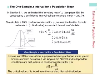
A confidence interval uses a sample statistic to estimate a population parameter. • In other words, a confidence interval uses a sample mean and standard deviation to estimate the population mean for that particular populations of interest. • But, since samples vary, the statistics we use, and thus the confidence intervals we construct, vary as well. Confidence Intervals
By the 68-95-99.7% Rule, we know • about 68% of all samples will have ’s within 1 SE of • about 95% of all samples will have ’s within 2 SEs of • about 99.7% of all samples will have ’swithin 3 SEs of • Consider the 95% level: • There’s a 95% chance that is no more than 2 SEs away from . • So, if we reach out 2 SEs, we are 95% sure that will be in that interval. In other words, if we reach out 2 SEs in either direction of , we can be 95% confident that this interval contains the true parameter mean. • This is called a 95% confidence interval. Confidence Intervals
The figure below shows that some of our 95% confidence intervals (from 20 random samples) actually capture the true mean (the green horizontal line), while others do not: True Mean () Confidence Intervals
Our confidence is in the process of constructing the interval, not in any one interval itself. • Thus, we expect 95% of all 95% confidence intervals to contain the true parameter that they are estimating. Confidence Intervals
We can claim, with 95% confidence, that the interval contains the true population mean. • The extent of the interval on either side of is called the margin of error (ME). • In general, confidence intervals have the form estimate ± ME. • The more confident we want to be, the larger our ME needs to be, making the interval wider. Margin of Error
To be more confident, we wind up being less precise. • We need more values in our confidence interval to be more certain. • Because of this, every confidence interval is a balance between certainty and precision. • The tension between certainty and precision is always there. • Fortunately, in most cases we can be both sufficiently certain and sufficiently precise to make useful statements. Margin of Error: Certainty vs. Precision
The choice of confidence level is somewhat arbitrary, but keep in mind this tension between certainty and precision when selecting your confidence level. • The most commonly chosen confidence levels are 90%, 95%, and 99% (but any percentage can be used). Margin of Error: Certainty vs. Precision (cont.)
The ‘2’ in (our 95% confidence interval) came from the 68-95-99.7% Rule. • Using a table or technology, we find that a more exact value for our 95% confidence interval is 1.96 instead of 2. • We call 1.96 the critical value and denote it z*. • We will discuss z* critical values at another time, as today we will focus on t* critical values. • For any confidence level, we can find the corresponding critical value (the number of SEs that corresponds to our confidence interval level). Critical Values
The sampling model found by William S. Gossethas been known as Student’s t. • The Student’s t-models form a whole family of related distributions that depend on a parameter known as degrees of freedom. • We often denote degrees of freedom as df, and the model as tdf. • When Gosset corrected the model for the extra uncertainty, the margin of error got bigger. • Your confidence intervals will be just a bit wider. • By using the t-model, you’ve compensated for the extra variability in precisely the right way. T – Model
As the degrees of freedom increase, the t-models look more and more like the Normal model. • In fact, the t-model with infinite degrees of freedom is exactly Normal. T – Model
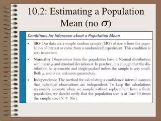
Conditions: • Independence Assumption: • Independence Assumption: The data values should be independent. • Randomization Condition:The data arise from a random sample or suitably randomized experiment. Randomly sampled data (particularly from an SRS) are ideal. • 10% Condition:When a sample is drawn without replacement, the sample should be no more than 10% of the population. Conditions and Assumptions (Important)
Normal Population Assumption: We can never be certain that the data are from a population that follows a Normal model, but we can check the… • Nearly Normal Condition:The sample data come from a distribution that is unimodal and symmetric. • Check this condition by making a histogram of raw data, if available. Otherwise, look for indications that the data follow a Normal distribution. • The smaller the sample size (n < 15 or so), the more closely the data should follow a Normal model. • For moderate sample sizes (n between 15 and 40 or so), the t works well as long as the data are unimodal and reasonably symmetric. • For larger sample sizes, the t methods are safe to use unless the data are extremely skewed. Conditions and Assumptions (cont.)
When the conditions are met, we are ready to find the confidence interval for the population mean, μ. • The confidence interval is where the standard error of the mean is = • The critical value depends on the particular confidence level, C, that you specify and on the number of degrees of freedom, n – 1, which we get from the sample size. One-Sample t-Interval for the Mean
Either use the table provided, or you may use your calculator: • Finding probabilities under curves: • normalcdf( is used for z-scores (if you know ) • tcdf( is used for critical t-values (when you use s to estimate ) • 2nd Distribution • tcdf(lower bound, upper bound, degrees of freedom) • Finding critical values: • 2nd Distribution • invT(percentile, df) Finding Critical t* Values
Practice calculating the critical t* values for the following using the table: • 95% confidence for a sample of 10 • 95% confidence for a sample of 20 • 95% confidence for a sample of 30 • 90% confidence for a sample of 57 • 99.5% confidence for a sample of 7 Finding Critical t* Values (cont.)
Check Conditions and show that you have checked these! • Random Sample: Can we assume this? • 10% Condition: Do you believe that your sample size is less than 10% of the population size? • Nearly Normal: • If you have raw data, graph a histogram to check to see if it is approximatelysymmetric and sketch the histogram on your paper. • If you do not have raw data, check to see if the problem states that the distribution is approximately Normal. • State the test you are about to conduct (this will come in hand when we learn various intervals and inference tests) • Ex) One sample t-interval • Show your calculations for your t-interval • Report your findings. Write a sentence explaining what you found. • EX) “We are 95% confident that the true mean weight of men is between 185 and 215 lbs.” Summary: Steps Finding t-Intervals
Amount of nitrogen oxides (NOX) emitted by light-duty engines (games/mile): Construct a 95% confidence interval for the mean amount of NOX emitted by light-duty engines. Finding t-Intervals
Given a set of data: • Enter data into L1 • Set up STATPLOT to create a histogram to check the nearly Normal condition • STAT TESTS 8:Tinterval • Choose Inpt: Data, then specify your data list (usually L1) • Specify frequency – 1 unless you have a frequency distribution that tells you otherwise • Chose confidence interval Calculate • Given sample mean and standard deviation: • STAT TESTS 8:Tinterval • Choose Stats enter • Specify the sample mean, standard deviation, and sample size • Chose confidence interval Calculate Finding t-Intervals in the Calculator
Interpretation of your confidence interval is key. • What NOT to say: • “90% of all the vehicles on Triphammer Road drive at a speed between 29.5 and 32.5 mph.” • The confidence interval is about the mean not the individual values. • “We are 90% confident that a randomly selected vehicle will have a speed between 29.5 and 32.5 mph.” • Again, the confidence interval is about the mean not the individual values. • “The mean speed of the vehicles is 31.0 mph 90% of the time.” • The true mean does not vary—it’s the confidence interval that would be different had we gotten a different sample. • “90% of all samples will have mean speeds between 29.5 and 32.5 mph.” • The interval we calculate does not set a standard for every other interval—it is no more (or less) likely to be correct than any other interval. Caution: Be sure to correctly interpret your Interval
DO SAY: • “90% of intervals that could be found in this way would cover the true value.” • Or make it more personal and say, “I am 90% confident that the true mean is between 29.5 and 32.5 mph.” Caution: Be sure to correctly interpret your Interval