Download
1 / 13
160 likes | 366 Views
Vertical Mixing. Sandstrom’s theorem requires an input of mechanical energy to drive the vertical circulation in the ocean. Where does this energy input come from ? Wind or tide ? Is it sensitive to climate change ? Does it have feedback potential ?. Agenda. Turbulence & mixing.

E N D
Vertical Mixing Sandstrom’s theorem requires an input of mechanical energy to drive the vertical circulation in the ocean. Where does this energy input come from ? Wind or tide ? Is it sensitive to climate change ? Does it have feedback potential ?
Agenda • Turbulence & mixing. • Methods for estimating mixing. • & identifying sources of mixing energy. • Internal Waves and Tides • What drives the mixing ? • The ongoing controversy: wind or tide mixing ?
Vertical Mixing • A result of turbulence. • The TKE equation: (assuming no transport) • P – the rate of production of TKE (ie. the rate of transfer of energy from the mean flow). • dj/dt – the of increase of water column potential energy. • e – the rate at which TKE is dissipated to heat. ie. energy transferred from mean flow is either dissipated to heat or used to increase water column PE (ie. mix).
June& Nov CTD profiles T S Estimating Vertical Mixing I • Kz the diffusion coefficient. Links the diffusive flux to the gradient of concentration. • Can be estimated from changes in concentration of conservative tracers (ambient salinity or addition of dyes, eg. SF6). • Provides a measure of the large scale mixing rate, but not source of mixing energy.
Dye-diffusion Experiments • SF6 : inert tracer, with very low detection limits. Not found in nature or pollution and is not toxic. • Oceanic values of Kz ~ 0.11-0.17 (North Atlantic). • ie. an order of magnitude smaller than Munk ! • Watson & Ledwell (2000, JGR, 105, 14325-14337). NATRE : Put time scale !
Estimating Vertical Mixing II • Via measurement of a turbulent parameter, the rate of dissipation, e. • This can then be related to mean flow, enabling identification of the source of the mechanical energy driving the mixing. • BUT in order to estimate the mixing rate, an efficiency, Rf is required. • From theory, values of 0.17 – 0.2 have been estimated. • Via a bulk parameterisation, ie. rate at which energy is dissipated by tidal friction. • Observed values range from 0.0037–0.06.
Brazil basin to Mid-Atlantic Ridge Ledwell et al. (2000, Nature, 403,179-182) Much enhanced mixing over mid-Atlantic Ridge compared to basin to west. Measurement of Dissipation • Can be related to the mean flow. • Individual profiles. Are they representative of the portion of ocean in which they are taken ? • Instantaneous profiles. Are they temporally representative ? • Gregg (1998, AGU Vol. 54, 305-338)
Internal Tides/ Waves • Stratified flow over sufficiently steep topography. • Energy transfer from the mean flow into internal wave motions. • These propagate away, dissipating and performing mixing. • Internal tides are common. • May be subject to dynamical constraints.
Stigebrandt fjord model • Fjords have deep basins cut-off from direct contact with the ocean for much of the time. At this time the deep water properties are only changed through mixing with overlying water. • Linear fit – Rf is no sensitive to the fjord geometry. ie. all energy going into fjord must be dissipated. • ie. dissipation must take place close to the sill. Stigebrandt & Aure (1989, JPO, 19,917-926) W – the observed rate of increase of water column potential energy (dj/dt). E – model estimated internal wave flux.
Applied the fjord to the Ocean. Used observed stratification and topography to estimate energy transfer to the internal tide Used Rf = 0.05 from fjord work to estimate rate of working in mixing the water column. The results suggest that a substantial proportion of the mixing required could be explained by the internal tide. Can this be tested ? Looking at the distribution of dissipation of tidal energy. The mixing must take place near to the IT generation point. Link the mixing to the internal tide. Stigebrandt Ocean Mixing Model
Distribution of Dissipation of Tidal Energy • It was thought that tidal energy was dissipated in shallow continental shelf seas. • Problem: estimates only accounted for 66% of the astronomical value. • Topex-Porsidon provides global estimates of sea surface height. • Assume local balance: W-P= dissipation W – rate of working by TGF. P – tidal energy flux (Topex) Egbert & Ray (2000, Nature, 405, 775-778). Estimates show significant amounts of mixing in deep ocean – over rough topography.
Evidence of ‘tidal’ mixing • Compiling the Brazil basin experiment data into a time series: there is a springs-neap cycle in the diffusivity. • Only the tides operated at these frequencies.
Wind Mixing • Surface wind mixing: - only affects the surface mixed layer. - therefore need to bring deep water to the surface to mix it. (Ekman suction in the Southern Ocean). • Inertial oscillations/ internal waves. - a dynamical mechanism to get wind energy dissipated on the surface into the deep water. • Difficult to link wind and mixing as there is no periodic signal.