The Goldilocks Problem

1. The Goldilocks Problem Tudor Hulubei Eugene C. Freuder Department of Computer Science University of New Hampshire Sponsor: Oracle

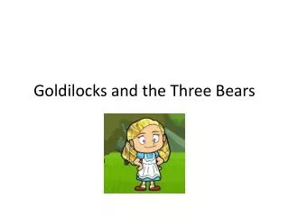
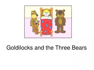
2. Introduction “So away upstairs she went to the bedroom, and there she saw three beds. There was a very big bed for Father bear, but it was far too high. The middle-sized bed for Mother bear was better, but too soft. She went to the teeny, weeny bed of Baby bear and it was just right.” -- Goldilocks and the Three Bears

3. Introduction(continued) • A lot of work in Constraint Satisfaction has been focused on finding solutions to hard problems. • Many problems of practical interest are not difficult, but have a huge number of solutions, few of which are acceptable from a practical standpoint. • We are proposing a value ordering heuristic that will guide the search towards acceptable solutions.

4. Motivation and Applications • Provide vendors with tools that can be used to suggest upgrades (upselling) and alternative solutions to customers. This can be achieved by combining a matchmaker or deep-interview strategy with our heuristic that guides the search towards acceptable solutions. • Provide a way for vendors to promote particular configurations, implement company policies, etc.

5. Example • Solution: v1=1, v2=1, v3=-1 • SW=(0.8+0.1+0.8)+(0.7+0.5)=2.9 • MinSW=(0.2+0.1+0.8)+(0.1+0.2)=1.4 • MaxSW=(0.8+0.7+0.9)+(0.9+0.5)=3.8 v1 v1={0=0.2, 1=0.8} v2={1=0.1, 2=0.7} v3={-1=0.8, 4=0.9} c12={(0,1)=0.1, (1,1)=0.7, (1,2)=0.9} c13={(0,-1)=0.2, (0,4)=0.3, (1,-1)=0.5} c13 c12 v2 v3

6. Definitions • Weights: • Represent “goodness”. • Are associated with: • every value in the domain of a variable. • every pair of allowed values in a constraint. • Solution Weight: • Defined as the sum, over all the variables and constraints, of the weights associated with the values and pairs of values involved. • Lower and upper limits : • MinSW (computed as the sum of the minimum weights of the values and pair of values in all the variables and constraints). • MaxSW (computed as the sum of the maximum weights of the values and pair of values in all the variables and constraints).

7. Definitions(continued) • Acceptable Solutions: • Given two positive real numbers MinASW and MaxASW (the minimum/maximum acceptable solution weight) s.t.: MinSW  MinASW  MaxASW  MaxSW, a solution is considered acceptable if: MinASW  SW  MaxASW. • The ideal solution weight (IdealSW) is defined as the center of the [MinASW,MaxASW] range. • Active Constraints: • During the search, a constraint is considered “active” if it involves at least one variable that has not yet been instantiated.

8. The acceptable-weight Heuristic • One way of looking for acceptable solutions is by parsing the entire search space and stop at the first solution whose weight is acceptable. • We can do better than that. We can guide the search towards solutions with acceptable weights, using a special value ordering heuristic called “acceptable-weight”. • The heuristic will dynamically compute the average of the individual weight (AIW) that the remaining variables and constraints would contribute to the global solution weight, should it equal IdealSW: ( IdealSW - SW(SolvedSubproblem) ) AIW = --------------------------------------------------------------------------------- (number of uninstantiated variables + number of active constraints)

9. The acceptable-weight Heuristic (continued) Past variables Current variable Future variables • The acceptable-weight heuristic will select the value that will minimize the absolute difference between SW” and IdealSW”. • After the assignment of v4, AIW is recomputed, to compensate for the amount we were off compared to the IdealSW”. v1={1=0.1}, v2={6=0.2}, v3={4=0.4}, v4={1=0.1, 5=0.8} c14={(1,1)=0.1, (1,5)=0.2} c24={(6,1)=0.8, (6,5)=0.9} c34={(4,1)=0.6, (4,5)=0.7} v1 [1] v5 [1,2] c14 c45 c24 c46 v2 [6] v4 [1,5] v6 [2,3] AIW=0.4  IdealSW”=(0.1+0.2+0.4)+AIW+3*AIW=2.3 Options for v4: v4=1: SW”=(0.1+0.2+0.4+0.1)+(0.1+0.8+0.6)=2.6 v4=5: SW”=(0.1+0.2+0.4+0.8)+(0.2+0.9+0.7)=3.3  The heuristic selects v4=1. c34 v3 [4] P”={{v1,v2,v3}, {c14,c24,c34}}. Note: v5 & v6 are not considered.

10. The acceptable-weight Heuristic(continued) • The strategy behind the acceptable-weight heuristic is two-fold: • Locally, we try to make sure that each subproblem centered around the current variable has a weight that is in line with the global IdealSW. • Globally, by constantly adjusting the AIW we try to control the overall deviation of the solution weight.

11. Experimental Results Variables: 100 Domain size: 5 Density: 0.00 Tightness: 0.00 Range size: 0.05 MAC range: 0.455-0.54 MAC+acceptable-weight range: 0.226-0.79 Variables: 100 Domain size: 5 Density: 0.00 Tightness: 0.25 Range size: 0.05 MAC range: 0.469-0.560 MAC+acceptable-weight range: 0.244-0.752

12. Experimental Results(continued) Variables: 100 Domain size: 5 Density: 0.00 Tightness: 0.25 Range size: 0.1 MAC range: 0.444-0.584 MAC+acceptable-weight range: 0.216-0.798 Variables: 100 Domain size: 5 Density: 0.055 Tightness: 0.25 Range size: 0.1 MAC range: 0.447-0.569 MAC+acceptable-weight range: 0.415-0.568

13. Experimental Results(continued) Variables: 100 Domain size: 5 Density: 0.0651 Tightness: 0.25 Range size: 0.1 MAC range: 0.43-0.55 MAC+acceptable-weight range: 0.44-0.54

14. Experimental Results(continued) Variables: 100 Domain size: 5 Difficulty peak for tightness=0.25 is at density=0.0651.

15. Future Work • Potential Improvements: • Look ahead, skip subtrees of the search space where an acceptable weight is not achievable. • Consider future variables when estimating the solution weight of the local subproblem centered around the current variable. • Avoid getting stuck in an interval when the heuristic doesn’t seem capable of escaping it.

16. Conclusions • The acceptable-weight heuristic presented here is designed to guide the search towards solutions with acceptable weights, when solutions can be ranked on a given dimension. • Experiments show that MAC+acceptable-weight guides the search towards acceptable solutions very quickly, much faster than MAC alone. • Even around the difficulty peak, MAC+acceptable-weight works well, slightly faster than MAC, with a very similar coverage.