Download
1 / 22
230 likes | 364 Views
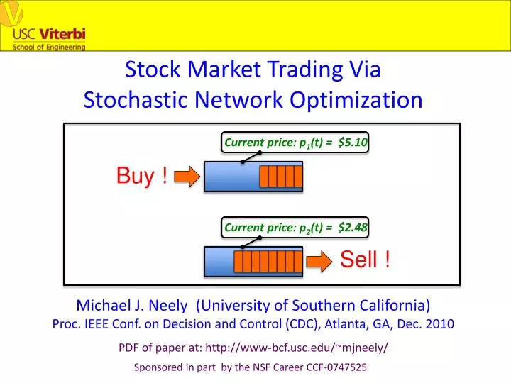
Stock Market Trading Via Stochastic Network Optimization. Current price: p 1 (t) = $5.10. Buy !. Current price: p 2 (t) = $2.48. Sell !. Michael J. Neely (University of Southern California) Proc. IEEE Conf. on Decision and Control (CDC), Atlanta, GA, Dec. 2010

E N D
Stock Market Trading Via Stochastic Network Optimization Current price: p1(t) = $5.10 Buy ! Current price: p2(t) = $2.48 Sell ! Michael J. Neely (University of Southern California) Proc. IEEE Conf. on Decision and Control (CDC), Atlanta, GA, Dec. 2010 PDF of paper at: http://www-bcf.usc.edu/~mjneely/ Sponsored in part by the NSF Career CCF-0747525
Problem Setting: • N stocks. • Slotted time t = {0, 1, 2, …}. • Prices p(t) = (p1(t), …, pN(t)). • Stock shares Q(t) = (Q1(t), …, QN(t)) Current price: p1(t) = $5.10 Buy ! Current price: p2(t) = $1.57 Buy ! Current price: p3(t) = $2.03 Sell !
Goal: Make money over time while limiting the • investment risk! • Limit risk by: • Bounding the max allowable stock level Qnmax. • Bounding the amount buy/sell on a slot. • Decision Variables for Buying: • An(t) = Num. shares of stock n bought on slot t. • bn(A) = Buying transaction fee (function of A). Current price = pn(t) Buy ! Expensen(t) = An(t)pn(t) + bn(An(t))
Goal: Make money over time while limiting the • investment risk! • Limit risk by: • Bounding the max allowable stock level Qnmax. • Bounding the amount buy/sell on a slot. • Decision Variables for Selling: • μn(t) = Num. shares of stock n sold on slot t. • sn(μ) = Selling transaction fee (function of μ). Current price = pn(t) Sell ! Revenuen(t) = μn(t)pn(t) - sn(μn(t))
Control Constraints and Decision Structure: • Buying Constraints: • An(t) in {0, 1, 2, …, μnmax} for all n, t. • ∑nAn(t)pn(t) ≤ xmaxfor all t. • Selling Constraints: • μn(t) in {0, 1, 2, …, μnmax} for all n, t. • μn(t) ≤ Qn(t) for all n, t. • Every slot t, observe prices p(t) = (p1(t), …, pN(t)). • Make buying/selling decisions. • Profit(t) = ∑nRevenuen(t) – ∑nExpensesn(t). • Want to maximize time average profit subject to • the above constraints.
Talk Outline: Design optimal strategy under (simplistic) assumption that price vectors p(t) are i.i.d. over slots. Use same strategy for arbitrary price vectors (assuming only that 0 ≤ pn(t) ≤ pnmax for all t). For arbitrary prices, show the strategy yields profit arbitrarily close to that of an “ideal” algorithm with perfect knowledge of future prices over T-slot frames (for any integer T). “T-slot lookahead metric”
Comparison to Related Work: • “Portfolio Optimization” • (Known or approximate price distributions) • [Markowitz 1952][Sharpe 1963][Samuelson 1969] • [Rudoy, Rohrs 2008] (Dynamic Programming) • 2) “Universal Portfolios” • (Arbitrary price sample paths) • [Cover 1991][Cover, Ordentlich 1996][Ordentlich, Cover 1998] • [Merhav, Feder 1993]
Comparison to Related Work: • Different Structure for Prior “Universal Portfolio” work: • Optimize “growth exponent.” • No cap on queue size (more aggressive, but more risk!) • Integer constraints relaxed to real numbers. • No Transaction fees. • Based on “Universal Data Compression.” • Solution complexity grows with time. • Comparison to ours: • Our cap on buy/sell and queue size limits risk, but • also limits to only linear growth (*not exponential). • Based on “Stochastic Network Optimization.” • Simple “max-weight” solution with complexity • that is the same for all time. • *simple modifications can get back exponential growth. $$ time
Solution Strategy: Dynamic Queue Control θn Qn(t) • Want to keep queue size high enough to take advantage of good prices that come along. • Don’t want queues too high (too risky). • Lyapunov Function: • L(Q(t)) = ∑n (Qn(t) – θn)2
Control Design: Qn(t) • Lyapunov Function L(Q(t)) • Lyapunov Drift Δ(t) = L(Q(t+1)) – L(Q(t)) • Every slot t, observe Q(t), p(t), and • minimize the drift-plus-penalty*: θn Δ(t) + V[Expenses(t) – Revenue(t)] *from stochastic network optimization theory [Georgiadis, Neely, Tassiulas 2006][Neely 2010] Results in the following algorithm: • (Selling) Choose μn(t)to solve: • Minimize: [θn– Qn(t) – Vpn(t)]μn(t) + Vsn(μn(t)) • Subject to: μn(t) in {0, 1, 2, …, min[Qn(t), μnmax]}
Control Design: Qn(t) • Lyapunov Function L(Q(t)) • Lyapunov Drift Δ(t) = L(Q(t+1)) – L(Q(t)) • Every slot t, observe Q(t), p(t), and • minimize the drift-plus-penalty*: θn Δ(t) + V[Expenses(t) – Revenue(t)] *from stochastic network optimization theory [Georgiadis, Neely, Tassiulas 2006][Neely 2010] Results in the following algorithm: • (Buying) Choose An(t)to solve: (“knapsack-like” problem) • Minimize: ∑n[Qn(t)-θn +Vpn(t)]An(t) + V∑nbn(Αn(t)) • Subject to: (already stated) constraints on (An(t)).
Theorem (iid case): Qn(t) Choose θn = V pnmax + 2μnmax. Then: μnmax≤Qn(t) ≤ Vpnmax+ 3μnmax(for all t) For all t: E{Time avg. Profit up to t} ≥ Profitopt– θn “Startup Cost” B L(Q(0)) – V Vt “Profit Gap” (c) As t infinity, we have with prob. 1: limtinfinity[Time avg profit] ≥ Profitopt – B/V
Now for arbitrary (possibly non-ergodic) prices: • Compare to an “ideal” T-slot lookahead metric. • ΨT[r] = Optimal Profit over frame r, assuming future stock prices over the frame are known. Frame 0 Frame 2 Frame 1
Now for arbitrary (possibly non-ergodic) prices: • Compare to an “ideal” T-slot lookahead metric. • ΨT[r] = Optimal Profit over frame r, assuming future stock prices over the frame are known. Frame 0 Frame 2 Frame 1 Metric even allows “selling short”
Theorem (General Bounded Prices): Under same algorithm as before: μnmax≤Qn(t) ≤ Vpnmax+ 3μnmax(for all t) For all frame sizes T>0, all integers R>0: Time average profit over RT slots ≥ - - CT L(Q(0)) 1 RTV V RT R-1 ∑r=0ΨΤ[r]
Simulations for BlockBuster Stock (BBI): Aug. 11, 1999 – Sept. 11, 2009 Avg Profit = Avg Profit on Trades - (1/t) x Startup Cost + (1/t) x Profit when sell all at end
Simulations for BlockBuster Stock (BBI): Aug. 11, 1999 – Sept. 11, 2009 Avg Profit = Avg Profit on Trades - (1/t) x Startup Cost + (1/t) x Profit when sell all at end “Asymptotically Negligible” as t infinity (But very significant for finite t !!!) • Parameters: μmax = 20,pmax = 30, V=1000 • Compare bound For T=10 (2 weeks), T=100 (20 weeks) : • Avg. Profit on trades ≥ “2-week ideal” – $2.0 • Avg. Profit on trades ≥ “20-week ideal” - $20.0
Simulations for BlockBuster Stock (BBI): Cumulative Trade Profit (Forward Time) Stock Prices (Forward Time) Average Profit Per Transaction = Cum. Trade Profit/t = $81.52 (2-week ideal profit no more than $30.00, 20-week idea profit no more than $60.00) Cumulative Trade Profit (Backward Time) Stock Prices (Backward Time) Average Profit Per Transaction = Cum. Trade Profit/t = $95.81
What about total profit (including startup costs)? • Forward Time: • Trade Profit = $206,343.20 • Startup Cost = $449,097.99 • End Reward = $33,976.80 • Total Profit = -$208,778.00 • Reverse Time: • Trade Profit = $242,512.40 • Startup Cost = $35,146.80 • End Reward = $239,499.00 • Total Profit = $446,864.60
What about total profit (including startup costs)? • Forward Time: • Trade Profit = $206,343.20 • Startup Cost = $449,097.99 • End Reward = $33,976.80 • Total Profit = -$208,778.00 • Reverse Time: • Trade Profit = $242,512.40 • Startup Cost = $35,146.80 • End Reward = $239,499.00 • Total Profit = $446,864.60
What about total profit (including startup costs)? • Forward Time: • Trade Profit = $206,343.20 • Startup Cost = $449,097.99 • End Reward = $33,976.80 • Total Profit = -$208,778.00 • Reverse Time: • Trade Profit = $242,512.40 • Startup Cost = $35,146.80 • End Reward = $239,499.00 • Total Profit = $446,864.60
Conclusion: • Provide a Lyapunov Optimization (“max-weight”) • approach to stock market trading. • Can quantify risk and profit guarantees compared to • T-Slot Lookahead: Time average profit over RT slots ≥ - - • Startup Cost is high and thus there is inherent risk, but • optimizing the trading profits mitigates this risk. • Open question: Can other algorithms provide provably better tradeoffs? CT L(Q(0)) 1 RTV V RT R-1 ∑r=0ΨΤ[r]