Download
1 / 47
470 likes | 1.01k Views
Lecture 7. Few points about earthquakes. Outline. Some basic facts and questions Great Chilean earthquake /Valdivia earthquake / of 1960 (Mw=9.5) and recent Tahoku earthquake (Mw=9.0) of 2011 Megathrust earthquakes and structure of the upper plate

E N D
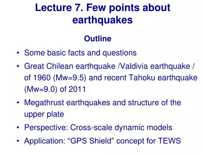
Lecture 7. Few points about earthquakes Outline • Some basic facts and questions • Great Chilean earthquake /Valdivia earthquake / of 1960 (Mw=9.5) and recent Tahokuearthquake (Mw=9.0) of 2011 • Megathrust earthquakes and structure of the upper plate • Perspective: Cross-scale dynamic models • Application: “GPS Shield” concept for TEWS
Some basic facts The cause of larger earthquakes is the plate tectonics and most of them happen at plate boundaries About 80% of relative plate motion on continental boundaries is accommodated in rapid earthquakes With few exceptions, earthquakes do not generally occur at regular intervals in time or space.
Some basic facts The shear strain change associated with large earthquakes (i.e. coseismic strain drop) is of the order of 10-5– 10-4. This corresponds to a change in shear stress (i.e. static stress drop) of about 1–10 MPa. The repeat times of major earthquakes at a given place are about 100–1000 years on plate boundaries, and 1000–10 000 years within plates.
Some basic facts Ideal Real
Some basic facts Deformation modes rare The magnitude–frequency relationship (the Gutenberg–Richter relation) log N(M) = a − bM, b is about 1
Some basic questions Why some plate boundaries glide past each other smoothly, while others are punctuated by catastrophic failures? Why do some earthquakes stop after only a few hundred meters while others continue rupturing for a thousand kilometers? How do nearby earthquakes interact? Why are earthquakes sometimes triggered by other large earthquakes thousands of kilometers away?
Valdivia earthquake (1960) Slip distribution
Region of Valdivia earthquake (1960) GPS data
Japan, 2011, Inverted Slip, m Tohoku Great Earthquake, 2011 (Mw=9.0) Japan, 2011, Fit of the co-seismic GPS data Model versus DART buoys data Tsunami based on source from GPS data inversion Hoechner et al. in prep
Song and Simons, Science, 2003 Wells et al.,JGR, 2003 Fuller et al., Geology, 2006
Megathrust earthquakes and structure of the upper plate Song and Simons, Science, 2003 Wells et al.,JGR, 2003
Correlation of large slip regions (asperities) with the negative gravity anomalies (sedimentary basins) Possible explanation (not convincing) Song and Simons, Science, 2003
Better explanation Fuller et al., Geology, 2006
Better explanation Fuller et al., Geology, 2006 However, this model should be recalculated including mantle lithosphere
Zones of seismicity Perspectives: Cross-scale dynamic models
Elastic deformation is included in our geological-time-scale (mln years) Andes model Full set of equations mass momentum energy
Frictional instabilities governed by static-kinetic friction Stress static friction stress kinetic friction Lc slip Slip Time The static-kinetic (or slip-weakening) friction: experiment Constitutive law Ohnaka (2003)
Frictional instabilities governed by rate- and state-dependent friction Dieterich-Ruina friction: At steady state: • were: • V and are sliding speed and contact state, respectively. • a, b and are non-dimensional empirical parameters. • Dc is a characteristic sliding distance. • The * stands for a reference value.
How b-a changes with depth ? • Note the smallness of b-a. Scholz (1998) and references therein
The depth dependence of b-a may explain the seismicity depth distribution Scholz (1998) and references therein
The central Andes model at geological time-scale Trench roll-back 18 Ma Delaminating lithosphere 0 Ma South American drift The Central Andes model Friction = 0.05 35 Ma Sobolev and Babeyko, Geology, 2005
We can continue calculation at seismic-cycle time-scale (years) 30
Modified FLAC = LAPEX (Babeyko et al, 2002) Dynamic relaxation: For geological-time-scale models ρiner>> ρ (ρ is real density). By taking ρiner= ρ we can model seismic waves
Rupture and seismic waves modeled with the Andes thermomechanical model Movy file waves.avi
Conclusions Large earthquake is still poorly understood phenomenon Observed correlation with the structure of the upper plate (not subducting plate) is surprising and intriguing The best (till now) explanation is stability of the wedge (Fuller at al, 2005), but thier model needs update Interesting perspective is a cross-scale modeling allowing simulation of seismic cycle or even rupture propagation in the same model that explains geological-time-scale processes
Bengkulu Max. wave heights for «southern» fault 37
Bengkulu Max. wave heights for «northern» fault 38
Epicenter and magnitude are the same.Not the same with tsunami impact in Bengkulu. 39
Siberut Padang Trench Bathymetry off Padang: An important player A A’ Bathymetry chart across the trench A’ A 40
The two scenarios are easily to distinguish by their GPS fingerprints Patch 1 Patch 2 43
Japan, 2011, Inverted Slip, m Tohoku Great Earthquake, 2011 (Mw=9.0) Japan, 2011, Fit of the co-seismic GPS data Model versus DART buoys data Tsunami based on source from GPS data inversion Hoechner et al. in prep
Japan, 2011, Inverted Slip, m Tohoku Great Earthquake, 2011 (Mw=9.0) Japan, 2011, Fit of the co-seismic GPS data
Concept of the “GPS-Shield” for Indonesia: Configuration and resolution Earthquake magnitude Sobolev et al., 2006, EOS Sobolev et al., 2007, JGR Location of maximum uplift 47