Download
1 / 32
330 likes | 473 Views
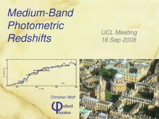
Photometric Redshifts. PHAT Meeting Pasadena 3-5 Dec 2008. Christian Wolf. data. model. Farb- bibliothek. estimator. Schätzer/ Klassifikator. Frequentist precision statistics: = “Using what IS there: N(z)!”. result. Bayesian frontier exploration: = “What do we (not) know: p(z)=?”.

E N D
Photometric Redshifts PHAT MeetingPasadena3-5 Dec 2008 Christian Wolf
data model Farb-bibliothek estimator Schätzer/Klassifikator Frequentist precision statistics:= “Using what IS there: N(z)!” result Bayesian frontier exploration:= “What do we (not) know: p(z)=?” Photo-z Ingredients & Application empirical data or external template 2-fitting artificial neural netlearning algorithms spectral energydistribution PDF: p(z)
Model + Estimator Combinations • 2 • PDF Ambiguity warning • NN • No PDF, no warning • Template model • Can be extrapolated in z,mag • Calibration issues • Priors’ issues • Empirical model • Good priors • No calibration issues • Can not be extrapolated Code 2 NN Model Template Empirical
PStar type ML PGalaxy redshift MEV PQuasar redshift Class Decision and z-Estimation <z> ± z Can include morphology etc.in statistics or neural net
Examples from COMBO-17 Classification ~98% complete at R<23 Stars (~3,000) White Dwarfs (~30) Ultra-cool WD (1) Galaxies (~30,000) QSOs (~300)
E colour z=0.52 z=0.56 Sb colour Redshift Error Regimes • Three regimes in photo-z quality • Saturation • Model-data calibration offsets in test causes p(z)-biases • Transition • Locally linear colour(z) grid • Breakdown • Globally nonlinear colour(z) grid mag
Galaxies: Saturation & Transition R=20 R=22 R=23.7 Galaxies at z~0.45
R=21.5 R=22.9 R=23.8 QSOs: Saturation at R<24 rms 0.008 7%-20%outlier QSOs at z~2.8
Catastrophic failures & misclassifications Large z errors Local z bias Unrealistic z errors Model ambiguities in colour space (spotted?) PDF too unconstrained PDF wrong (calib, prior) Mismatch between data and model Photo-Z Trouble
Catastrophic failures & misclassifications Large z errors Local z bias Unrealistic z errors Model ambiguities in colour space PDF too unconstrained PDF wrong (calib, prior) Mismatch between data and model Add more data Add model priors Repair modelsor calibration Realistic data errors Common Fixes
Add More Data: Wider Range • Wider coverage • Covers spectral features across wider z range • Add NIR data • For z > 1 galaxies • Only weak & high-variance features in rest-frame UV • Red z>1 galaxies with noisy optical data • Add UV data (e.g. GALEX) • For QSOs (Ball et al. 2007) • Lyman break at z < 2-3 Abdalla et al. 2007
z/(1+z) ~ 0.006 z/(1+z) ~ 0.015 QE (%) Wolf, Gray & Meisenheimer 2005 Wolf et al. 2004 λ/ nm Add More Data: Narrow Filters • Improve localization and contrast of features • QSO line detection avoids catastrophic failures at z < 3 • Galaxies+QSOs: improve z • Galaxy, star, QSO, WD,… ? Wolf 2001
S/N high p prior q p S/N medium q p S/N low q Add Priors… • Impact: ptot = pprior pcolour • Reduce rate of catastrophic failures (bimodal PDF) • Reduce larger z (up to √2) • Explicit for template models • Luminosity function, range • Mag / z extrapolation ~”ok” • ANN prior = training sample • Restricted in mag & z • Mag extrapolation wrong • Z extrapolation impossible • Spectroscopic selection?
Repair (or Make) Templates Budavari et al. 2000,2001
Kinney et al. templates 25% z outliers Age Abell 901 z~0.16 Dust Wolf, Gray & Meisenheimer 2005 Repair Models: Uncommon Objects • COMBO-17 field Abell 901/2 • Super-cluster at zspec~ 0.16 • 800 members with R < 21 • Photo-z 2002: using SEDs by Kinney et al. (1996) • 25% of S/N~100 members outliers with zphot~ 0.06 • z ~ 0.1 SHOCK! • Red spirals! • Photo-z 2003: include dust-reddened old SEDs • ~1% outliers
Photometry: PSF-matched Calibration (obs. frame) Artefacts: instrumental, data reduction Error distribution, non-Gaussian systematics in Gaussian error floor Source variability Stars: RR Lyr, long-term Galaxies: supernovae Photometric Blends Transient blends by moving objects Close neighbours Line-of-sight projections, strong lenses Binaries, WD+M etc. SED composition AGN component Composite stellar populations Photometry & SEDs
Basic method: Assume Gaussian PSF Convolve to worst PSF Photometry in aperture A Problems: Local PSF variations Non-Gaussian PSF (Capak et al. 2007) Special case: Gaussian aperture Stronger weight to brighter object centre Aeff = PSF A(“space-based aperture”) If A and PSF Gaussian, then Aeff Gaussian as well Minimize computations:Fix Aeff &adjust A to PSF 2A = 2eff - 2PSF (Röser & Meisenheimer 1991) Non-gaussian aperture Shapelet-based method(Kuijken 2008) PSF-Matched Photometry
What We Understand by Now • Origin of local z bias • Observed-frame + rest-frame calibration • Non-flat priors, positive-defined redshift • Origin of catastrophic outliers • Unrecognised z ambiguity in colour space • Wrong SED data and errors: e.g. blends • Minimum z variance levels • Intrinsic SED variations • Spectral resolution
E colour z=0.52 z=0.56 Sb colour Local Z Bias: Calibration • N = number of filters, i.e. independent data points • Calibration offsets in N=3 D • 1-D normalisation • 1-D z-bias • 1-D restframe SED bias • 1 out of N offset dimensions causes a photo-z bias z • More filters smaller z (proj. component ~1/√N) • Narrow filters small z (larger col/z on feature) • Spectroscopy with N~102..3: z without flux calibration • Few-filter photo-z’s limited by calibration accuracy • Many-filter photo-z’s limited by number and resolution of filters
Local Z Bias: Non-Flat Prior • Example: MegaZ-LRG (Collister et al. 2007) • Slope 1 in zspec-zphot • Mean z/(1+z)~0.03 • Contaminated with 5% stars (or 2% with shape data)
Local Z Bias: Non-Flat Prior • Assume • PDF p(z|colour) correct • Prior P (z) correct • dP/dz 0 • Or even P(z) = 0 at z<0 • Result • Expectation value z locally biased • Using = p(z|colour) rms • z = dP/dz p prior z However: Only in z = f(zspec) Not in z = f(zphot)
Catastrophic Outliers • Result from undetected ambiguities: Also: wrong data/errors • Example: see shrinking training sample • 20% sample in 1:20 ambiguities causes overall 1% unflagged outliers
Intrinsic Variety: Z Error Support • Example: • QSO near g-r~1 or z~3.7 • Main signal: Ly forest in g • Training sample in box • Redshift distribution:mean 3.66, rms 0.115 • RMS/(1+z) = 0.024 • Testing sample in box • RMS/(1+z) error 0.023 • Slope dz/d(g-r) relevant for noisy testing objects
What To Work On: Data • Define most effective & efficient data sets: • From simulations (…which don’t rule out outliers) • Describe data correctly: • Consistent apertures across bands • True photometric scatter by object • Minimiseunrecognised error sources in data: • Error floor from photometric blends & transients
What To Work On: Models • Templates etc.: • Best templates, rare objects with “different SEDs” • Best priors, best extrapolation in (mag, z) • Training samples: • Discretization effects, confidence limits on random-ness • Propagation into n(z) errors and outlier risks • Derive size requirements • Combine all approaches? • Empirical + extrapolated template model for all kinds of use
Galaxies: No Ambiguities ANN 2 template 2 empirical Collister & Lahav 2004 ~0% outliersz/(1+z)>0.1 rmsz/(1+z) = 0.023 Bias ~0.00 ~4%outliersz/(1+z)>0.1 rmsz/(1+z) = 0.042 Bias -0.017 ~0% outliersz/(1+z)>0.1 rmsz/(1+z) = 0.020 Bias ~0.00
QSOs: Strong Ambiguities ANN 2 template 2 empirical Filipe A. ~12% outliersz/(1+z)>0.3 rmsz/(1+z) = 0.113 Bias ~0.00 ~22%outliersz/(1+z)>0.3 rmsz/(1+z) = 0.056 Bias +0.015 ~1% outliersz/(1+z)>0.3 rmsz/(1+z) ~ 0.04 Bias ~0.000
flux / qef 1000 nm 400 nm Redshift Errors & Resolution • Objects at different redshifts • Filterset 's fixed z = 0.843 G2 star vs.QSO z=3 z = 1.958 z = 2.828