Download
1 / 22
280 likes | 1.17k Views
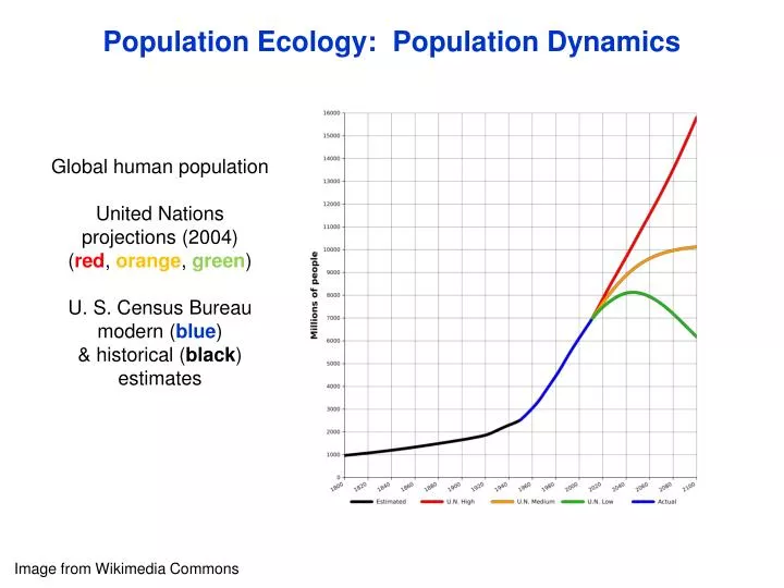
Population Ecology: Population Dynamics. Global human population United Nations projections (2004) ( red , orange , green ) U. S. Census Bureau modern ( blue ) & historical ( black ) estimates. Image from Wikimedia Commons. Population Dynamics.

E N D
Population Ecology: Population Dynamics Global human population United Nations projections (2004) (red, orange, green) U. S. Census Bureau modern (blue) & historical (black) estimates Image from Wikimedia Commons
Population Dynamics The demographic processes that can change population size: Birth, Immigration, Death, Emigration B. I. D. E. (numbers of individuals in each category) For an open population, observed at discrete time steps: = Nt + B + I – D – E Nt+1 For a closedpopulation, observed through continuous time: dN = (b-d)N dt dN = rN dt (b-d) can be considered a proxy for average per capita fitness
Population Dynamics 5 main categories of population growth trajectories: Exponential growth Logistic growth Population fluctuations Regular population cycles Chaos
Population Dynamics Deterministic logistic growth Invariant density-dependent vital rates dN N 1 – = rN dt r K Stable equilibrium carrying capacity Cain, Bowman & Hacker (2014), Fig. 11.5
Population Dynamics Deterministic vs. stochastic logistic growth Invariant density-dependent vital rates “Fuzzy” density-dependent vital rates r ri Stable equilibrium carrying capacity Fluctuating abundance within a range of values for carrying capacity Cain, Bowman & Hacker (2014), Fig. 11.5
Population Dynamics Time lags can cause delayed density dependence, which can result in population cycles If r is small, logistic Instead of growth tracking current population size (as in logistic), growth tracks density at units back in time If r is intermediate, damped oscillations dN N(t-) 1 – = rN dt K If r is large, stable limit cycle Cain, Bowman & Hacker (2014), Fig. 11.10
Population Dynamics Time lags can cause delayed density dependence, which can result in population cycles or chaos Sir Robert May, Baron of Oxford Photo from http://www.topbritishinnovations.org/PastInnovations/BiologicalChaos.aspx
Population Dynamics Population cycles&chaos Population size (scaled to max. size attainable) Per capita rate of increase
Variation in rand population growth Is the long-term expected per capita growth rate (r) of a population simply an average across years? Consider this hypothetical example: rgood = 0.5; rbad = -0.5 If the numbers of good & bad years are equal, is the following true? rexpected = [rgood + rbad] / 2 At t0, N0=100 t1 is a bad year, so N1 = N0 + (rbad* N0) = 50 t2 is a good year, so N2= N1 + (rgood*N1) = 75 The expected long-term r is clearly not 0 (the arithmetic mean of rgood & rbad)!
Variation in and population growth Nt+1 = Nt Nt+1 = Nt A fluctuating population Arithmetic mean = 1.02 Geometric mean = 1.01 1.21 0.87 1.17 1.02 1.13 Cain, Bowman & Hacker (2014), Analyzing Data 11.1, pg. 258
Variation in and population growth Nt+1 = Nt Nt+1 = Nt A steadily growing population 1.02 1000 Arithmetic mean = 1.02 1.02 1020 Geometric mean = 1.02 1.02 1040 1.02 1061 1.02 1082 1.02 1104 1.02 1126 1148 Cain, Bowman & Hacker (2014), Analyzing Data 11.1, pg. 258
Variation in and population growth Nt+1 = Nt Nt+1 = Nt A steadily growing population 1.01 1000 Arithmetic mean = 1.01 1.01 1010 Geometric mean = 1.01 1.01 1020 1.01 1030 Which mean (arithmetic or geometric) best captures the trajectory of the fluctuating population (the example given in the textbook)? 1.01 1040 1.01 1051 1.01 1061 1072 Cain, Bowman & Hacker (2014), Analyzing Data 11.1, pg. 258
Population Size & Extinction Risk Small populations are especially prone to extinction from both deterministic and stochastic causes Deterministic r < 0 Genetic stochasticity& inbreeding Demographic stochasticity individual variability around r(e.g., variance at any given time) Environmental stochasticity temporal fluctuations of r(e.g., change in mean with time) Catastrophes
Population Size & Extinction Risk Demographic stochasticity Each student is a sexually reproducing, hermaphroditic, out-crossing annual plant. Arrange the plants into small sub-populations (2-3 plants/pop.). In the first growing season (generation), each plant mates (if there is at least 1 other individual in the population) and produces 2 offspring. Offspring have a 50% chance of surviving to the next season. flip a coin for each offspring; “head” = lives, “tail” = dies. Note that average r = 0; each parent adds 2 births to the population and on average subtracts 2 deaths [self & 1 offspring – since 50% of offspring live and 50% die] prior to the next generation.
Population Size & Extinction Risk Environmental stochasticity How could the previous exercise be modified to illustrate environmental stochasticity?
Population Size & Extinction Risk Natural catastrophes What are the likely consequences to populations of sizes: 10; 100; 1000; 1,000,000 if 90% of individuals die in a flood?
Population Size & Extinction Risk Allee Effects occur when average per capita fitness declines as a population becomes smaller Birth (b) ? Rate ? Death (d) K Density (N) Zone of AlleeEffects
Spatially-Structured Populations Patchy population (High rates of inter-patch dispersal, i.e., patches are well-connected)
Spatially-Structured Populations Mainland-island model (Unidirectional dispersal from mainland to islands)
Spatially-Structured Populations Classic Levins-type metapopulation (collection of populations) model (Vacant patches are re-colonized from occupied patches at low to intermediate rates of dispersal ) Assumptions of the basic model: occupied 1. Infinite number of identical habitat patches occupied 2. Patches have identical colonization probabilities (spatial arrangement is irrelevant) unoccupied unoccupied 3. Patches have identical local extinction (extirpation) probabilities occupied 4. A colonized patch reaches K instantaneously (within-patch population dynamics are ignored) occupied Original metapopulation idea from Levins (1969)
Spatially-Structured Populations Classic Levins-type metapopulation (collection of populations) model (Vacant patches are re-colonized from occupied patches at low to intermediate rates of dispersal ) dp = cp(1 - p) - ep occupied dt p = proportion of patches occupied occupied unoccupied c = patch colonization rate e = patch extinction rate unoccupied occupied Key result:metapopulation persistence requires (e/c)<1 occupied Original metapopulation idea from Levins (1969)
Source-Sink Population Dynamics Habitats vary in habitat quality; occupied sink habitats broaden the realized niche sink source source source sink sink Original source-sink idea from Pulliam (1988)