Download
1 / 149
1.5k likes | 1.68k Views
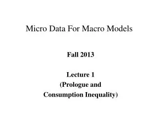
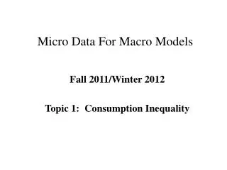
Micro Data For Macro Models. Topic 2: Consumption Inequality and Lifecycle Consumption. Part A: Background on Household Surveys (Jonathan Covered This in TA Sessions). Micro Expenditure Data: Household Surveys. Consumer Expenditure Survey (U.S. data) Starts in 1980

E N D
Micro Data For Macro Models Topic 2: Consumption Inequality and Lifecycle Consumption
Part A:Background on Household Surveys(Jonathan Covered This in TA Sessions)
Micro Expenditure Data: Household Surveys Consumer Expenditure Survey (U.S. data) Starts in 1980 Broad consumption measures Some income and demographic data Repeated cross-sections Panel Study of Income Dynamics (U.S. data) Starts in late 60s Only food expenditure consistently Housing/utilities (most of the time) Broader measures (recently) Very good income and demographics Panel nature
Micro Expenditure Data: Household Surveys British Household Panel (British Data) o Panel data including income and expenditure Family Expenditure Survey (British Data) Bank of Italy Survey of Household Income and Wealth (Italian Data) o Panel data including income and expenditure There are others….many Scandinavian countries, Japan, Canada, etc. Even some developing economies have detailed household surveys that track some measures of consumption (e.g., Mexico, Taiwan, Thailand)
Micro Expenditure Data: Scanner Data Nielsen Homescan Data o Large cross-section of households o Very detailed level transaction data (at the level of UPC code) o Some demographics o Some panel component o Matches quantities purchased with prices paid o Covers most of the large MSAs o Measurement error? o Selection? o Coverage of goods?
Micro Income Data: Household Surveys Current Population Survey (CPS) o Usual data set used within U.S. to track labor supply and earnings. o Has panel component. o Can be found at www.ipums.org/cps/ PSIDCan be found at http://psidonline.isr.umich.edu/ Survey of Income and Program Participation (SIPP) o Four year rotating panel o Large sample sizes o Over samples poor Census/American Community Survey o Can be found at www.ipums.org
Income and Consumption Inequality Large literature documenting the increase in income inequality within the U.S. during the last 30 years (Katz and Autor, 1999; Autor, Katz, Kearney, 2008) Consumption is a better measure of well being than income (utility is U(C) not U(Y)). Does income inequality imply consumption inequality? Depends on whether income inequality is “permanent” Depends on insurance mechanisms available to households Depends on other margins of substitution (home production, female labor supply, etc.).
Why Do We Care About Consumption Inequality? Why is it important? o Learn about well being over time (economic growth, standard of livings, inequality, etc.). o Learn about insurance mechanisms available to households (public insurance, private insurance, etc.)? o Learn about the nature of income processes (more on this in the next set of lecture notes).
A Classic: Attanasio and Davis (1996) A Short Discussion: The innovation of the Attanasio and Davis technique. The creation of synthetic cohorts from cross sectional data.
Krueger and Perri (2006) What they do: o Use data from the Consumer Expenditure Survey (CEX) to track the evolution of consumption inequality. o CEX is includes a nationally representative sample of households. - Designed to compute consumption weights for CPI - Short panel dimension (4 quarters) - Mostly used as repeated cross sections. - Includes detailed spending measures on expenditures by categories. o Use repeated cross sections to track consumption inequality.
Krueger and Perri (2005): What They Conclude Conclusions o Income inequality is much greater than consumption inequality o If some of the increase in income inequality is idiosyncratic, households can self insure (or public sector can provide insurance) making consumption inequality respond less than income inequality. o Write down a model where insurance is endogenously provided. Increasing idiosyncratic shocks to income can increase demand for insurance (leading to more insurance). Consistent with their model, credit card access increased during this period. o Bottom line: Use the consumption data to learn about the nature of income processes and insurance mechanisms.
Part D:Revisiting Trends in Consumption Inequality Accounting for Measurement Error in Data
Can Measurement Error Alter Inequality Findings? Yes Depends on whether measurement error differs across the consumption (income) distribution. Suppose richer households have been underreporting their income to a greater extent in recent periods (relative to the past). The rich could be increasing their expenditure more (relative to other parts of the distribution). However, the systematic measurement error could also be increasing. How to test for group specific differences in measurement error?
Aguair and Bils (2011) Try to account for differential measurement error over different “income-demographic” groups to get a sense of changing consumption inequality. Some particulars: Define xijt = average expenditure on good j, by group i, at time t j goods = food at home, clothing, utilities, entertainment, etc. i groups = cells based on income (5) and demographics (18) DefineXit= average total expenditure for group i at time t. Formally:
The Essence of the Exercise (From a Discussion by Jonathan Parker; NBER EFG 2011) Log budget share of good: lnwi = ln (xi /X ) Inferred 2006 Observed 2006 Estimated Engel curve for luxury Observed 1980 Inferred adjustment to ln X90 Estimated Engel curve for normal good Log total real expenditure: X = xLux+xNormal+xNec ln X90 ln X90 ln X10 ln X90 ln X10
Aguair and Bils (2011) Assume measurement error in expenditure…… represents a good specific error (common across all groups) represents a group specific error (common across all goods)
Aguair and Bils (2011): Some Intuition Difference-in-Difference Estimates (2 good case, 2 group case) Goods = e (entertainment) and f(food) Groups = high (rich) and low (poor) (difference out good specific error) (difference out good specific error)
Aguair and Bils (2011): Some Intuition Take differences across goods to eliminate group specific error Obtain an unbiased estimate of relative consumption inequality. Need to map into units of total expenditure. Want to recover:
Aguair and Bils (2011) Suppose for true expenditures, x*: Can estimate the following using actual data in some period 0 where systematic measurement error is less of an issue: If there is no measurement error in the data, can uncover: Assumes income elasticities are constant over time (and can be locally estimated). Assume measurement error is zero in period 0.
Aguair and Bils (2011): Some Intuition Substituting in the estimated β’s, we get:
Relative Spending Differences Between High and Low Income Groups Aguiar and Bils (2011) Findings
Different Saving Rates From the CEX Aguiar and Bils (2011) Findings
Attanasio, Hurst, and Pistaferri (2012) Also show that measurement error likely results in the underestimation of changes in consumption inequality within the U.S. Like Aguiar and Bils, find that consumption inequality and income inequality have moved essentially one-for-one over the past thirty years. Use other empirical approaches and data sets. You can find a copy of the paper on my web page (under working papers).
Attanasio, Hurst, and Pistaferri (2012) • Use CE Diary Data (a separate survey) as opposed to CE Interview Data (which was • used by Krueger/Perri and Aguiar/Bils. • Diary data found to have less measurement error (better matches NIPA trends).
Attanasio, Hurst, and Pistaferri (2012) • Imputed PSID Consumption matches income inequality nearly identically. • Food PSID Consumption also matches income inequality trends (need to scale by • food income elasticity which is about 0.5).
Conclusions: Part 1 (A – D) Measurement error is important in Consumer Expenditure Survey! Even though there is measurement error, can still measure consumption inequality. Without controlling for measurement error, looks like small increases in consumption inequality. Much of that is due to the rich reporting less and less of their expenditures. Controlling for the systematic recent underreporting of the rich increases the estimated consumption inequality in the U.S. to levels that match the changing income inequality.
Why Do We Care About Lifecycle Expenditure? Why is it important? Learn about household preferences broadly C.E.S. vs. log vs. other / Habits? / Status? - Estimate preference parameters intertemporal elasticity of substitution/ risk aversion/ discount rate - Learn about income process permanent vs. transitory shocks / expected vs. unexpected - Learn about financial markets/constraints liquidity constraints / risk sharing arrangements - Learn about policy responses spending after tax rebates, fiscal multipliers, etc.
Why Do We Care (continued)? The big picture with consumption: - Use estimated parameters to calibrate models - Understand business cycle volatility - Conduct policy experiments (social security reform, health care reform, tax reform, etc.) - Estimate responsiveness to fiscal or monetary policy - Broadly understand household behavior
How We Will Proceed The outline of the next part of the lecture: - Understand lifecycle consumption movements o Illustrative of how one fact can spawn multiple theories. o Show how a little more data can refine the theories o Illustrate the empirical importance of the Beckerian consumption model (i.e, incorporating home production and leisure).
Fact 1: Lifecycle Expenditures Plot: Adjusted for cohort and family size fixed effects
Define Non-Durable Consumption (70% of outlays) • Use a measure of non-durable consumption + housing services • Non-durable consumption includes: Food (food away + food at home) Entertainment Services Alcohol and Tobacco Utilities Non-Durable Transportation Charitable Giving Clothing and Personal Care Net Gambling Receipts Domestic Services Airfare • Housing services are computed as: Actual Rent (for renters) Imputed Rent (for home owners) – Impute rent two ways • Exclude: Education (2%) , Health (6%), Non Housing Durables (16%), and Other (5%) <<where % is out of total household expenditures>>