Mass Flux in a Horizontally Homogeneous Atmosphere A useful tool for emissions and lifetimes.

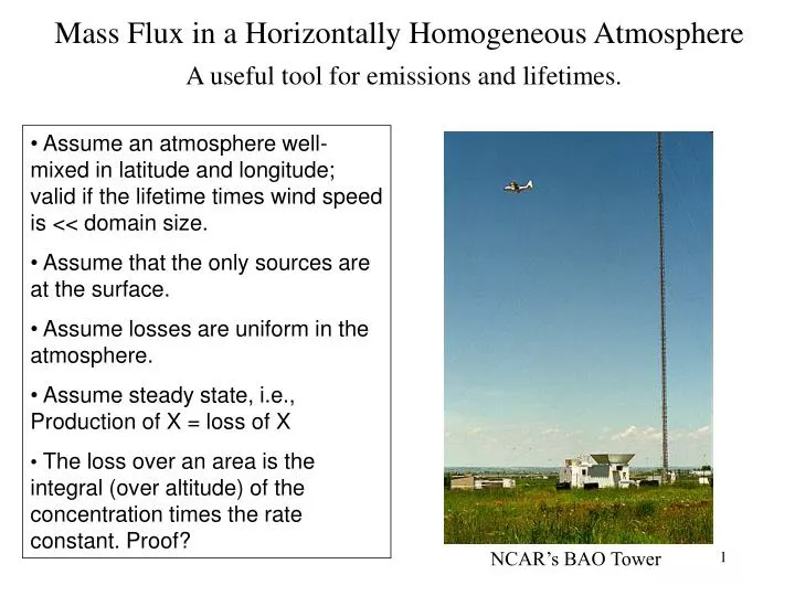
1. Mass Flux in a Horizontally Homogeneous AtmosphereA useful tool for emissions and lifetimes. • Assume an atmosphere well-mixed in latitude and longitude; valid if the lifetime times wind speed is << domain size. • Assume that the only sources are at the surface. • Assume losses are uniform in the atmosphere. • Assume steady state, i.e., Production of X = loss of X • The loss over an area is the integral (over altitude) of the concentration times the rate constant. Proof? NCAR’s BAO Tower

2. View from the top of the BAO tower

3. For a trace species X with an exponential decay with altitude, the column content, WX, is the altitude integral.If H0 (m) is the scale height for concentration in gm-3 then: For altitude profiles that do not follow a clean exponential decay, the column content must be measured.

4. If X is in steady state then production equals loss. Production = Flux of X (g m-2 s-1) Loss = Where k’ = first order rate (or pseudo first order) constant (s-1) X = concentration (g m-3) For an exponentially decaying species:

5. Example of NO over a fertilized corn field. NOZ = NO0e(-Z/600)

6. In the this example H0 = 600 m and WX = 6x10-5 g m-2. Production = Flux of X (g m-2 s-1) Loss Production = Flux = k’ WNO Let X be NO over a large fertilized corn field at night. The only loss is reaction with O3. NO + O3→ NO2 + O2 If k = 2x10-14 cm3 s-1 and [O3] = 50 ppb, then [O3] >> [NO] and k’ = 2x10-14 x 50x10-9 x2.5x1019 = 2.5x10-2 s-1 Flux = k’ WNO = 2.5x10-2 s-1 x 6x10-5 = 1.5x10-6 g m-2 s-1. Enough to generate ozone photochemically.

7. Example 2. Profiles of SO2 over the eastern US. • SO2 has little impact on weather or climate, but sulfate aerosols do. How fast is SO2 oxidized to sulfate? • The main source of SO2 is coal combustion for electricity generation, and the emission rates are reasonably well known. • The known sinks are dry deposition, attack by OH, and oxidation to sulfate in clouds containing aqueous H2O2, but the strength of these sinks remains uncertain. • The effective lifetime tnet is:

8. The average profile measured from aircraft shows that most of the SO2 resides below 3000 m altitude. CMAQ SO2 column content is 1.5 times larger than the observed column content. CMAQ and aircraft SO2

9. CMAQ Aircraft Example comparison.The Good: Smallest 5% differences between CMAQ and aircraft.

10. CMAQ Aircraft The not so bad: Median differences between CMAQ and aircraft.

11. CMAQ Aircraft The Ugly: Largest 95% differences between CMAQ and aircraft.

12. GOCART and Aircraft GOCART average SO2 column content is 1.4 times larger than the aircraft column content.

13. SO2 lifetime • The SO2 profile shows a rapid decrease with altitude, nearing zero by 3000 m. • If SO2 is destroyed before it is advected away from the source, we can assume steady state conditions. • Production of SO2 = loss of SO2 • The loss over an area is the integral (over altitude) of the concentration times the rate constant. Production = Flux of SO2 (g m-2 hr-1) Loss k’ = first order rate constant (hr-1) [SO2] = concentration of SO2 (g m-3)

14. SO2 lifetime Production (Flux) = Loss Rearrange to get lifetime, t.

15. To test this theory we used a Gaussian plume dispersion model. Gaussian plume for a single point source.

16. Lifetimes and sources SO2 lifetimes (hours) generated using Gaussian plume dispersion model. Assumed lifetime = 4 hours. SO2 point sources SO2 lifetimes (hours) 0 -2 2 -6 6-17 17-47 47-620

17. Boxes for flux calculation Box 1 Box 2 Box 3 Power plants Boxes used to determine SO2 flux from point sources.

18. Lifetimes calculated assuming a 16 hour lifetime. 16 hr lifetime stats Add error (2 hours) and standard deviation in quadrature to get uncertainty of method = 2.8 hours

19. 24 hour back trajectories The flux from each US state and Canadian municipality was weighted by the number of back trajectory points that crossed the area.

20. Weighted flux from US states and Canadian municipalities (g hr-1m-2) . SO2 column content (g m-2) Uncertainty = (.952 + 2.82).5 = 3 hours

21. Summary • The average SO2 lifetime calculated using 180 measured profiles (from the summer in the Mid-Atlantic region) and EPA and Environment Canada emissions was 18 +/- 6 hrs (95% C.I.). • CMAQ and GOCART over-predict SO2 by 20 – 40% near the surface → The simulated lifetime is too long. Possible explanations: • Errors in cloud cover – leading to less reaction of SO2 and H2O2 in clouds. • Some unaccounted-for sink.