Download
1 / 34
340 likes | 480 Views
Neurophysiological significance of the inverse problem its relation to present “source estimate” methodologies and to future developments. E. Tognoli. Discussion group about Source Estimation 5 November 2004. I. A “poor spatial resolution”. EEG : a poor spatial resolution. Priors :

E N D
Neurophysiological significance of the inverse problemits relation to present “source estimate” methodologies and to future developments E. Tognoli Discussion group about Source Estimation 5 November 2004
EEG : a poor spatial resolution • Priors : • We are repeated that EEG has a “poor spatial resolution”, although good temporal one : thus, assumptions on structure-to-function are loose
Let’s localize the sources • Each of these 3 topographic maps comes from a single dipole activation of the cortex in a dipole simulator program. Estimate the locations of these 3 single sources
Volume conduction • Principe of EEG recording: volume currents • What you want to know: where (projected on scalp) something is happening • What you get: a large ususally bipolar propagation of the “source” • Effect : Blurs the signal
Anisotropy • Anisotropy : density/impedance of tissues • distort the topography of the signal recorded from the scalp, as compared to the signal recorded from the cortex • Act as a spatial low-pass filter • Effect : Blurs the signal
More of anisotropy • The sinuses: partially filled with… nothing • Effect : displaces the signal
Brain folding • Brain folding : the EEG signal mainly originates from pyramidal layers III & V. • The orientation of the active patch of neuron is of prime importance for the projection of the activity onto the electrodes • Effect : displaces the signal
Brain folding Source: Van Essen, 1997
“poor spatial resolution”? • Blurring of the source • Anisotropy • Volume conduction • Displacement of the source • Cavities • Brain folding • The signal is corrupted both in its extent and in its location
Some solutions? If pretending to do some topographical analysis of the EEG: • Because of this corrupted correspondence between the sources of bioelectrical activity and their scalp topography, we are lead to work, not in the space of the electrodes (maps/splines of raw signals), but in the space of the currents (maps/splines of estimated sources of raw signal) • We do not record directly the cortex, but do as if, with a mathematical reconstruction
Some solutions? • Solutions has been proposed through either : • Mathematical transform (eg. Laplacian, CSD) • Estimation/modeling (minimization of Laplacian in 3D (voxel-based) models : inverse problem)
Some solutions? • Solutions has been proposed through either : • Mathematical transform (eg. Laplacian, CSD) • Estimation/modeling (minimization of Laplacian in 3D (voxel-based) models : inverse problem)
Some solutions? • The Laplacian is problematic for spatial analysis of EEG data (eg. coherence analysis), since it projects correlated activities in 2 (presumably silent) unrelated locations of a tangential foci : source and sink • Although these data can be correctly interpreted (at least for a few sources), they lead to incorrect assumption of the structure-to-function relationship in the literature
Some solutions? • Solutions has been proposed through either : • Mathematical transform (eg. Laplacian, CSD) • Estimation/modeling (minimization of Laplacian in 3D (voxel-based) models : inverse problem)
Some solutions? • Estimation of sources : 2 approaches • Dipole: one single (or a few) point-like sources, center of mass of localized activity) : not useful for spectral/coherence analysis : information is excessively reduced • Smooth current estimates (reconstruction of time series at many (N’>N) spatial locations by estimating solutions to the inverse problem)
Some solutions? • No unique solution to the inverse problem • Under-determination (ill-posed problem) • Two crucial points for the accuracy of the estimation • Performance/assumptions of the algorithm (given an undetermined, noisy signal) • Accuracy of the head model
Algorithms • Inverse problem with smooth solution • MN (or MNE - minimum norm estimate, or LE, linear estimation) (Hamalainen & Ilmoniemi, 1984) • WMN (weight the contribution of sources regarding depth, to rule out the bias toward high contribution from sources close to the surface) • LORETA (low resolution electromagnetic tomography)- generalized weighted minimum norm/laplacian : extend the properties of MN by projecting solutions in true 3D (VOXEL BASED)(Pascual-Marqui) • VARETA (variable resolution electric-magnetic tomography) (Valdes-Sosa) • WROP (weighted resolution optimization) ; then LAURA (local autoregressive averages) (Grave de Peralta Menendez, 1997 ; 1999
Algorithms • Inverse problem with smooth solution • More details in the next sessions
Spline/head model I • The spline support of the transform/estimation : ( legacy of Laplacian/CSD) • Hjorth, 1975 • Perrin, 1987 • Law, 1995 • Babiloni, 1998
Spline/head model I • The spline support of the transform/estimation : ( legacy of Laplacian/CSD) • Hjorth, 1975 • Perrin, 1987 • Law, 1995 • Babiloni, 1998
Spline/head model II • Configuration of sulci and gyri (orientation of active cortical columns) • Realistic (MRI-based) models • FEM: extracts volumes of homogenous conductivity. • BEM : extracts boundaries between shells (typically, scalp, skull, CSF, brain)
Increasing accuracy of the shells • Typically now, 4 compartments: scalp, skull, CSF, grey matter
The accuracy of the estimated conductivities • Typically, models use average conductivity values (sampled in the literature) • Idiosyncrasy of the conductivity • In a given compartment, variability of the conductivity
The accuracy of the estimated conductivities • Anisotropy is a major contributor : • We can estimate (voxel-by-voxel) the conductivity with EIT (Electrical Impedance Tomography) • inject small current wave of known properties • record resulting waves • since current take the path of least impedance, it’s possible to compute, from the resulting wave (shape distortion and temporal variations) the distribution of conductivities. • Minimal equipment, then extensive mathematical modeling • Used for both anatomical and functional purposes