1 / 0

Lecture 4: The Fundamental Conservation Laws

Lecture 4: The Fundamental Conservation Laws. Weather Analysis Forecasting Ch. 4. Outline. The Hydrostatic Equation The Thickness Equation Conservation of Mass Conservation of Momentum Conservation of Energy. Introduction.

apollo
Download Presentation

Lecture 4: The Fundamental Conservation Laws

An Image/Link below is provided (as is) to download presentation Download Policy: Content on the Website is provided to you AS IS for your information and personal use and may not be sold / licensed / shared on other websites without getting consent from its author. Content is provided to you AS IS for your information and personal use only. Download presentation by click this link. While downloading, if for some reason you are not able to download a presentation, the publisher may have deleted the file from their server. During download, if you can't get a presentation, the file might be deleted by the publisher.

E N D

Presentation Transcript


  1. Lecture 4: The Fundamental Conservation Laws

    Weather Analysis Forecasting Ch. 4
  2. Outline The Hydrostatic Equation The Thickness Equation Conservation of Mass Conservation of Momentum Conservation of Energy
  3. Introduction Study of the physical world tends to be focused on the quantities such as mass, momentum, and energy. The behavior of the atmosphere is no exception to this rule. In these lecture notes, we will investigate the manner in which these quantities and their various interactions serve to describe the building blocks of a dynamical understanding of the atmosphere at middle latitudes.
  4. Distribution of Mass in the Atmosphere Recall that mass can be described as the measure of the substance of an object. The pressure exerted by Earth’s atmosphere decreases with increasing distance away from the surface as the depth of the fluid decreases. This implies that the mass of the atmosphere also decreases with height.
  5. Hydrostatic Equation Therefore, there is a vertical pressure gradient force given by The vertical pressure gradient force is largely balanced by the gravitational force For an atmosphere at rest, the net vertical force is zero, giving
  6. Hydrostatic Equation This expression is known as the hydrostatic equation and it represents the fundamental vertical balance condition in the Earth’s atmosphere. Hydrostatic balance is obeyed to great accuracy under nearly all conditions in the Earth’s atmosphere.
  7. Thickness Container the unit area column of atmosphere contained between 1000 hPa and 500 hPa. The mass of a 500 hPa, unit area slab is unique, but its depth varies day to day. This geometric depth is referred to as the thickness between two isobaric surfaces.
  8. Thickness Less (more) dense air will correspond to a greater (smaller) thickness. Less (more) dense air will correspond to a higher (lower) average temperature. Therefore, the thickness should have a bearing on the thickness between two isobaric levels.
  9. Thickness
  10. Thickness Equation Using the ideal gas law, the hydrostatic equation can be rewritten as Integrating this expression between pressure levels and at which the heights are and , we obtain This expression is known as the thickness equation, or the hypsometric equation
  11. Thickness Equation We can express the thickness equation in terms of a quantity called the geopotential. The geopotential is defined as the work required to raise a unit mass a distance dzabove sea level. Therefore, geopotential is given as Using this expression, we can rewrite the thickness equation as
  12. Applications of the Thickness Equation We will often refer to geopotential height (Z) in subsequent discussions and map analysis. The geopotential height is simply given by The thickness equation allows us to make a general relationship between temperature and geopotential heights on isobaric maps. As a rule, warmer temperatures in the lower troposphere imply higher geopotential heights at upper levels.
  13. Applications of the Thickness Equation
  14. Applications of the Thickness Equation
  15. Applications of the Thickness Equation One of the most common analysis products used to characterize and understand the weather is a sea level pressure map. In geographical regions characterized by high terrain, such as the Rocky Mountains of North America, the elevation is so far above sea level that use of the station pressure does not effectively contribute to this goal. In such regions the thickness equation can be used to calculate a reduced sea-level pressure, which is an estimate of what the sea-level pressure would be were the surface elevation 0 m.
  16. Altimeter Equation We begin with the thickness equation Let and be the desired values at sea level and let and be the observed station values. Rearranging the thickness equation gives us Solving for the gives the altimeter equation
  17. Altimeter Equation
  18. Mass Continuity Equation Consider an infinitesimal cube, fixed in space, through which air flows. Using the hydrostatic equation, we can write the control volume as The Lagrangian rate of change of mass (per unit mass) is given by
  19. Mass Continuity Equation Applying the chain rule gives This can be simplified to Writing the above expression in vector form gives the mass continuity equation
  20. Mass Continuity Equation Physically, the mass continuity equation states that regions of local convergence (divergence) leads to an increase (decrease) in mass. The mass continuity equation also demonstrates that horizontal convergence (divergence) leads to rising (sinking) motion in the atmosphere.
  21. Convergence and Vertical Motion
  22. Convergence and Vertical Motion
  23. Conservation of Momentum Newton’s 2nd law is a statement of the conservation of momentum As discussed previously, the five major forces that impact atmospheric motion are the Pressure Gradient Force Gravitational Force Viscous Force Centrifugal Force Coriolis Force Here, we will discuss the frictionless momentum equations
  24. Vertical Momentum Equation In order to construct a vertical equation of motion we must take account of all the forces with components in the local vertical direction. The relevant forces are: (1)The vertical pressure gradient force (2) The effective gravitational force (3) The vertical component of the viscous force We can write a first approximation to the vertical momentum equation as
  25. Vertical Momentum Equation For synoptic-scale motions, Therefore, the dominant balance will be between the vertical pressure gradient force and the gravitational force (i.e. hydrostatic balance). To first order, the atmosphere is in hydrostatic balance vertically.
  26. Horizontal Momentum Equations In order to construct a horizontal momentum equations, we must take account of all the forces with components in the local zonal and meridional directions. The relevant forces are: (1)The horizontal pressure gradient force (2) The Coriolis force We can write a first approximation to the horizontal momentum equations in vector form as
  27. Horizontal Momentum Equations In order to recast this expression in isobaric coordinates, we must convert the pressure gradient force term into an equivalent expression in isobaric coordinates. This is done by considering the differential on a constant pressure surface: Since there’s no change in pressure on an isobaric surface, then so that
  28. Horizontal Momentum Equations Next, we expand as a function of x and y to yield This can be rearranged into Since this statement is true for all dx and dy, this implies that
  29. Horizontal Momentum Equations Using the hydrostatic equation and dividing by ρ gives Therefore, the isobaric coordinate expression for the pressure gradient force in vector form is
  30. Horizontal Momentum Equations With the previous result, the vector form of the horizontal momentum equations can be rewritten as Here, For synoptic-scale motions, the dominant balance will be between the horizontal pressure gradient force and the Coriolis, leading to a balance condition called geostrophic balance.
  31. Momentum Equations A scaling analysis of the momentum equation for synoptic-scale motions show The two dominant vertical forces are the vertical pressure gradient force and gravitational force, leading to hydrostatic balance The two dominant horizontal forces are the horizontal pressure gradient force and the Coriolis force, leading to geostrophic balance
  32. Momentum Equations
  33. Conservation of Energy For macroscopic systems, the principle of energy conservation can be expressed through the first law of thermodynamics. The first law of thermodynamics for a moving air parcel can be written as This equation is known as the thermodynamic energy equation. The terms on the RHS represent the change in the internal energy of the system and the work done on the environment. This conversion process enables the solar heat energy to drive the motions of the atmosphere.
  34. Temperature Advection and Vertical Motion For adiabatic, steady-state, and stably stratified atmospheric flow, it can be shown that the thermodynamic energy equation can be written as Here is a measure of static stability This expression states that the horizontal temperature advection is related to the vertical motion such that warm (cold) air advection is associated with upward (downward) vertical motions.
  35. Temperature Advection and Vertical Motion
  36. Temperature Advection and Vertical Motion
  37. Potential Temperature An additional variable of meteorological consequence which arise from further consideration of the thermodynamic energy equation is the potential temperature It is the temperature a parcel of air would have it were adiabatically compressed (or expanded) from its original pressure, p, to a reference pressure, (usually 1000 hPa).
  38. Uses of Potential Temperature Potential temperature can be used to compare the temperature of air parcels that are at different levels in the atmosphere and can be used to predict temperature advection. If the potential temperature of an air parcel at one pressure level is colder than air parcels at other pressure levels, a forecaster can infer cold advection at the pressure level with the lowest potential temperature.
  39. Example
  40. Example
  41. Summary The reduced set of equations that describe the synoptic-scale atmosphere are given below
More Related