Download
1 / 45
450 likes | 570 Views
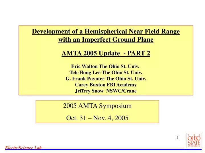
Development of a Hemispherical Near Field Range with an Imperfect Ground Plane AMTA 2005 Update - PART 2 Eric Walton The Ohio St. Univ. Teh-Hong Lee The Ohio St. Univ. G. Frank Paynter The Ohio St. Univ. Carey Buxton FBI Academy Jeffrey Snow NSWC/Crane. 2005 AMTA Symposium

E N D
Development of a Hemispherical Near Field Rangewith an Imperfect Ground PlaneAMTA 2005 Update - PART 2Eric Walton The Ohio St. Univ. Teh-Hong Lee The Ohio St. Univ.G. Frank Paynter The Ohio St. Univ.Carey Buxton FBI AcademyJeffrey Snow NSWC/Crane 2005 AMTA Symposium Oct. 31 – Nov. 4, 2005
THE TEAM: Dr. Eric K. Walton The Ohio State Univ., Columbus, OH Dr. Teh Hong Lee, The Ohio State Univ., Columbus, OH Carrey Buxton; FBI Academy, Quantico, VA Jeff Snow; Naval Surf. Weap. Ctr, Crane Labs., Crane, IN
THE PROBLEM The gain patterns of VHF/UHF antennas on structures that sit adjacent to the ground are influenced by the characteristics of the ground. Typical ground conductivity is such that VHF/UHF signals propagate significantly into the ground. The test and measurement of such antennas are more accurate with a test chamber that incorporates an imperfect ground. BUT: Normal spherical mode expansion techniques will not work in such an environment. APPROACH: A plane wave synthesis algorithm will be used along with an “outside the sphere” ground reflection term. Note that this is our 2nd annual talk on this topic.
GROUND REFLECTIONS IN NF MEASUREMENTS • SUMMARY/ INTRODUCTION • The Ohio State University ElectroScience Laboratory, the Naval Surf. Weap. Ctr, Crane Labs, Crane, IN are working to build a near field antenna measurement range. • The range is optimized for ground vehicles and thus is built as a hemispherical scanning system over a realistic roadway/ground surface. • The chamber size is 12.2 m high by 17.7 m wide by 21.3 m long. It will have absorber covered walls and ceiling with requirements from VHF to S-band.
GROUND REFLECTIONS IN NF MEASUREMENTS • THE BASIC CHAMBER • The surface of the chamber is a layer of concrete over a pit filled with damp sand 3 m deep. • To avoid asymmetry, the concrete will not have metal reinforcement bars. • The test vehicles will be driven onto an “H” frame so that the wheels rest on small metal pads connected to a central pivot. It will be lifted and rotated only 3 cm above the surface of the ground. This avoids the reflections from the edge of a large drive-on turntable that is sometimes used in such test ranges.
GROUND REFLECTIONS IN NF MEASUREMENTS SAND PIT
GROUND REFLECTIONS IN NF MEASUREMENTS • The probe positioning system • THETA: Steel arm connected to a central pivot • PHI: vehicle will rotate on the turntable while the arm moves in an arc. • The turntable and the arm move continuously. There is no stopping and starting of the two positioners. • Each frequency domain data point will be at a different position. This will require that the software transformations from the near field data to the far field must take these positional increments vs. frequency into account.
GROUND REFLECTIONS IN NF MEASUREMENTS • Transformation Software • The typical method of transforming from the near field to the far field consists of taking advantage of the efficiency of the Fourier transform. • The data are transformed into a spectrum of plane waves in the geometrical system to be used. • plane wave spectral components; • cylindrical wave components • spherical waves
GROUND REFLECTIONS IN NF MEASUREMENTS • HISTORY: • Probe corrected near-field scanning on a spherical surface was first solved in 1970 by Jensen in a doctoral dissertation at Technical University of Denmark. • Much of the history of near field scanning and transformation development is given in a 1988 special issue of the IEEE AP-S Transactions (V. 36, No. 6, June 1988).
RAY PATHS GROUND REFLECTIONS IN NF MEASUREMENTS • We are doing a hemispherical scan over an imperfect ground. • We do not have a complete set of spherical data. • since the ground is not perfectly reflecting, we cannot create a full set of spherical probe points by imaging. • We have collected all of the data that would propagate to the far field, however. Thus, we have a full set of data.
GROUND REFLECTIONS IN NF MEASUREMENTS • For this reason, we have chosen to perform the transformation from the near field to the far field by using a direct transformation (plane wave synthesis). • We define the far field direction and integrate (sum) the measurement over the lit zone of the measurement hemisphere. • We take polarization effects into account during this process. • Each test frequency has an associated set of test points, and must be summed independently. • This process does not permit the efficiencies associated with using Fourier (or cylinderical or spherical) components in an expansion, so the process is very inefficient. Modern very high speed computers will permit the transformations to be done in reasonable time.
RAY PATHS GROUND REFLECTIONS IN NF MEASUREMENTS The propagation from the vehicle to the far field point however can be by a direct propagation path, a ground reflection inside the probing zone, or a reflection outside of the probing zone.
GROUND REFLECTIONS IN NF MEASUREMENTS Thus the ray paths to consider when computing the far field: Possible Ray Paths from the Probe Zone to the Far Field. We have confirmed with borehole measurements of the dielectric properties of the sand that the loss in the sand is enough to mask reflections from the bottom of the pit. (“What goes in does not come out”.)
GROUND REFLECTIONS IN NF MEASUREMENTS MEASUREMENT POINTS
GROUND REFLECTIONS IN NF MEASUREMENTS Amplitude of the Probe Data Over a Hemisphere (omnidirectional probe antenna case)
GROUND REFLECTIONS IN NF MEASUREMENTS More Complex ...
GROUND REFLECTIONS IN NF MEASUREMENTS • Next compute the Far Field pattern due to the AUT model • Given the probe data points (/2; arrays) • And given the value (complex) of E(,) for each & • For a chosen set of far field angles (ff and ff arrays) • Compute sum over “lit” region:
Hemispherical NF Probing(with ground bounce effects) Radius = 4 m; Freq. = 0.7 GHz
GROUND REFLECTIONS IN NF MEASUREMENTS Far Field Azimuthal Patterns at 15 degrees elevation. (exact, direct, ground reflected, and sum)
Hemispherical NF Probing(with ground bounce effects) Radius = 3 m; Freq. = 0.7 GHz
Hemispherical NF Probing(with ground bounce effects) Radius = 2 m; Freq. = 0.7 GHz
Hemispherical NF Probing(with ground bounce effects) Radius = 3 m; Freq. = 0.95 GHz
Hemispherical NF Probing(with ground bounce effects) Radius = 5 m; Freq. = 0.4 GHz
2004 CONCLUSIONS • It is necessary to consider external ground reflections to obtain accurate FF patterns from NF probe data. • We have developed a NF to FF algorithm that separately computes the direct signal, the ground reflected signal and the sum signal. • It is necessary to make assumptions about the ground reflection coefficient in order to accurately compute the FF patterns (of course this is in the case where there is significant ground reflection outside the domain of the probe hemisphere)
GROUND REFLECTIONS IN NF MEASUREMENTS • 2004 CONCLUSIONS (cont) • WE ARE DESIGNING A GROUND VEHICLE NF ANTENNA MEASUREMENT RANGE • WE BELIEVE THAT HEMISPHERICAL PROBING ABOVE A REALISTIC GROUND CAN BE DONE • THE TRANSFORMATION FROM THE NF TO THE FF MUST INCLUDE THE EXTERNAL GROUND REFLECTION
Hemispherical NF Probing(with ground bounce effects) • 2005 WORK • Complete the NF to FF algorithm development for the omnidirectional probe data in order to explore the behavior of the algorithm • Include probe correction in the algorithm development work. • Include full polarization development work in the algorithm development work. • Begin the deliverable software development with an initial transition of the algorithm to the C++ programming.
Dipole AUT Volume SUPPORT ARM INTERACTIONS Single dipole: Figure 1. Probe supporting arm and AUT for the hemispherical near field measurement system.
ARM INTERACTION 3 ele. array • Studies involved various probe types and arm shapes. • Spurious signals can be reduced to better than 25 dB below the direct signals even at the lowest frequencies. Performance is better at the higher frequencies. (c) (d) Figure 14. Scattered field of supporting arm from the illumination of a 3-element x-directed dipole array located 28’ above the ground plane at 150 MHz. Phi=0 (x-z) plane cut.
MOIST SAND STUDY Dielectric constants of sands with various moisture content.
MOIST SAND STUDY(borehole example) 3 m; w &w/o PEC (a) dielectric constant (b) reflection coefficients Dielectric constant and the reflection coefficients of sample C1TOPA obtained from the proposed site of the facility. BOTTOM LINE: “WHAT GOES IN, STAYS IN”
PROBE INTERACTIONWITH FLOOR • Probe Interaction Study Conclusions • The difference between the ESP/MOM and BSC/PO results are due to evanescent coupling between the dipole and ground. • The difference becomes very small when the antenna is more than 0.5 l above the ground. • Nyquist sampling requirement for near field probing only requires that we use data down to 0.5 l above the ground. • Therefore, we believe that evanescent coupling in the NSWC-Crane hemispherical NF range will not cause significant errors. • We will still need a slot in the ground to permit the longer elements of the log-periodic antenna to extend below ground level so the shorter elements (higher frequency region) can still approach to within 0.5 l of the ground. • We believe a narrow thin slot is the best approach to accommodate the log-periodic antenna near the ground.
AUT to far field Surface of ground Radiating elements Synthesized Plane Wave Wavefront Synthesized below-ground elements (green) Individual spatial displacements PLANE WAVE SYNTHESIS Sketch of plane wave synthesis geometry.
Z FF tp P tf Ff Pf Y delf ff fp Ft X Pt PLANE WAVE SYNTHESIS Geometry for the near field to far field transformation
PLANE WAVE SYNTHESIS EXAMPLE RESULTS • Consider a single horizontal dipole. • oriented in the x-direction • 1.2 feet (0.366 meters) above a lossy dielectric half space. • relative permittivity = 2.75 • loss tangent = tan (δ) = 0.042. • frequency of operation = 500 MHz (wavelength = 60 cm) • probe hemisphere radius is 12 feet (3.66 meters). • The raw probe data was synthesized using a geometrical theory of diffraction computer code written by Dr. Ron Marhafka at the ESL (called NEC-BSC). • The near field to far field transformation was written in MATLAB.
(b) (a) (c) PLANE WAVE SYNTHESIS THEORETICAL Exact far field pattern results for the ½ wave dipole. (a. at φ = 0 degrees, (b) at φ = 45 deg. (c) at φ = 90 deg.
(a) (b) (c) Click quickly PLANE WAVE SYNTHESIS RESULT OF TRANSFORMATION Result of transformation to the far field; E-theta and E-phi vs. Theta (a) Phi = 0 deg.; Phi = 45 deg., Phi = 90 deg.)
GUI-BASED C++ PACKAGE“CRANE BENCH” This algorithm was passed to Frank Paynter, to develop a C++ GUI based package • SOFTWARE PACKAGE • PRIMARY GOALS: • Interactive; user-friendly • ASCII-formatted near field probe data • Display • analyze • SUB-GOALS • Interactive via mouse clicks • use the widely-supported MS Windows ‘look and feel’ • simple ASCII data formats • transform hemispherical near field probe data into far field • plot the results in a number of ways.
CRANEBENCH(by Frank Paynter) Crane DDAS Workbench User Interface
INTERESTING EXAMPLE(probe data) E-theta E-phi E-r • H-dipole; 1.2 ft. above realistic gnd; • 7 ft. offset in x direction • 12 ft. radius scanner; 500 MHz; • (note non-zero r-component)
INTERESTING EXAMPLE NOTE THE RECOVERED SYMMETRY
INTERESTING EXAMPLE(FAR FIELD RESULT) E-theta E-phi
CONCLUSIONS • WE HAVE DEVELOPED AN ALGORITHM FOR TRANSFORMATION FROM THE NF TO THE FF OVER A REALISTIC GROUND • WE HAVE PORTED THE ALGORITHM FROM MATLAB (development) TO C++ (user GUI) • WE HAVE TESTED THE ALGORITHM FOR VARIOUS STRESSFUL CASES AND ARE DEVELOPING RULES OF THUMB FOR THE USER (SET UP PARAMETERS AND ACCURACY ESTIMATES)
QUESTIONS ? Dr. Eric K. Walton, The Ohio State Univ. Dr. Teh Hong Lee, The Ohio State Univ. G. Frank Paynter The Ohio State Univ. Carey Buxton, FBI Academy Jeff Snow; NSWC/Crane HEY ! IS THAT A HEMI ?