Download
1 / 25
250 likes | 335 Views
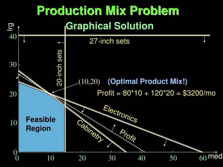
lrg. Production Mix Problem. 40. 27-inch sets. 30. 20-inch sets. (Optimal Product Mix!). (10,20). Profit = 80*10 + 120*20 = $3200/mo. Graphical Solution. 20. Electronics. Feasible Region. 10. Cabinetry. Profit. 0. med.

E N D
lrg Production Mix Problem 40 27-inch sets 30 20-inch sets (Optimal Product Mix!) (10,20) Profit = 80*10 + 120*20 = $3200/mo Graphical Solution 20 Electronics Feasible Region 10 Cabinetry Profit 0 med 0 10 20 30 40 50 60
Product Mix Problem Production Capacity Constraints: 6*med + 15*lrg < = 360 4*med + 5*lrg < = 140 med > = 0; lrg > = 0 (hours/set)*sets = hours Primal Problem Formulation Market Constraints: med < = 15 lrg < = 40 (sets) Objective Function: Maximize: Profit = 80*med + 120*lrg ($/set)*sets = $
Primal Problem(Interpretation of Dual Prices) Row Dual Price (Marginal value of an 1 1.000000 additional unit of 2 2.666667 the resource) 3 16.00000 4 0.0000000 5 0.0000000
Work-Scheduling Problem Define variables: Let xi = number of employees beginning work on day i, i = 1,…,7 Write objective function: Min z = x1 + x2 + x3 + x4 + x5 + x6 + x7 Impose constraints: x1 + x4 + x5 + x6 + x7 > 17 (Monday) x1+ x2 + x5 + x6 + x7 > 13 (Tuesday) x1+ x2 + x3 + x6 + x7 > 15 (Wednesday) x1+ x2 + x3 + x4 + x7 > 19 (Thursday) x1+ x2 + x3 + x4 + x5 > 14 (Friday) x2 + x3 + x4 + x5 + x6 + x7 > 16 (Saturday) x3 + x4 + x5 + x6 + x7 > 11 (Sunday) xi > 0 (i= 1, …, 7) (Non-negativity) Formulate as Linear Programming Problem
Work-Scheduling Problem MIN = @SUM( EMPLOYEES: NHIRED); @FOR( NEEDS( I): @SUM( EMPLOYEES( J): CONSTRAINTS( I, J) * NHIRED( J)) >= NREQUIRED( I)); ! We want NHIRED to be integer; @FOR(EMPLOYEES(I): @GIN(NHIRED(I))); END (LINGO Model: with Integer Constraint)
Work-Scheduling Problem Optimal solution found at step: 8 Objective value: 23.00000 Branch count: 1 Variable Value NHIRED( MONDAY) 7.000000 1.000000 NHIRED( TUESDAY) 3.000000 1.000000 NHIRED( WEDNESDAY) 2.000000 1.000000 NHIRED( THURSDAY) 7.000000 1.000000 NHIRED( FRIDAY) 1.000000 1.000000 NHIRED( SATURDAY) 3.000000 1.000000 NHIRED( SUNDAY) 0.0000000 1.000000 (LINGO Solution: with Integer Constraint)
Allocation of Scarce Resources, II Powerco, Electrical Power Company Power Transmission Costs: ($/million kwh) To Supply From City 1 City 2 City 3 City 4 (million kwh) Plant 1 $8 $6 $10 $9 35 Plant 2 $9 $12 $13 $7 50 Plant 3 $14 $9 $16 $5 40 Demand 45 20 30 30 Transportation Problems
Transportation Problem Define Variables: Let Xij = number of (million kwh) produced at plant i and sent to city j. Objective Function: Min z = 8*X11 + 6*X12 + 10*X13 + 9*X14 + 9*X21 + 12*X22 + 13*X23 + 7*X24 + 14*X31 + 9*X32 + 16*X33 + 5*X34 Powerco Power Plant: Formulation Supply Constraints: X11 + X12 + X13 + X14 < = 35 (Plant 1) X21 + X22 + X23 + X24 < = 50 (Plant 2) X31 + X32 + X33 + X34 < = 40 (Plant 3)
Transportation Problem Demand Constraints: X11 + X21 +X31 > = 45 (City 1) X12 + X22 +X32 > = 20 (City 2) X13 + X23 +X33 > = 30 (City 3) X14 + X24 +X34 > = 30 (City 4) Powerco Power Plant: Formulation (Cont’d.) Nonnegativity Constraints: Xij > = 0 (i=1,..,3; j=1,..,4) Balanced? Total Demand = 45 + 20 + 30 + 30 = 125 Total Supply = 35 + 50 + 40 = 125 Yes, Balanced Transportation Problem! (If problem is unbalanced, add dummy supply or demand as required.)
Transportation Problem model: ! A 3 Plant, 4 Customer Transportation Problem; SETS: PLANT / P1, P2, P3/ : CAPACITY; CUSTOMER / C1, C2, C3, C4/ : DEMAND; ROUTES( PLANT, CUSTOMER) : COST, QUANTITY; ENDSETS ! The objective; [OBJ] MIN = @SUM( ROUTES: COST * QUANTITY); Powerco Power Plant: LINGO Formulation
Transportation Problem ! The demand constraints; @FOR( CUSTOMER( J): [DEM] @SUM( PLANT( I): QUANTITY( I, J))>= DEMAND( J)); ! The supply constraints; @FOR( PLANT( I): [SUP] @SUM( CUSTOMER(J): QUANTITY(I,J))<=CAPACITY( I)); ! Here are the parameters; DATA: CAPACITY = 35, 50, 40 ; DEMAND = 45, 20, 30, 30; COST = 8, 6, 10, 9, 9, 12, 13, 7, 14, 9, 16, 5; ENDDATA end Powerco Power Plant: LINGO Formulation (Cont’d.)
Transportation Problem Optimal solution found at step: 7 Objective value: 1020.000 QUANTITY( P1, C1) 0.0000000 QUANTITY( P1, C2) 10.00000 QUANTITY( P1, C3) 25.00000 QUANTITY( P1, C4) 0.0000000 QUANTITY( P2, C1) 45.00000 QUANTITY( P2, C2) 0.0000000 QUANTITY( P2, C3) 5.000000 QUANTITY( P2, C4) 0.0000000 QUANTITY( P3, C1) 0.0000000 QUANTITY( P3, C2) 10.00000 QUANTITY( P3, C3) 0.0000000 QUANTITY( P3, C4) 30.00000 Powerco Power Plant: LINGO Solution All Quantities are Integers!
Transportation Problem Row Slack or Surplus Dual Price OBJ 1020.000 1.000000 DEM( C1) 0.0000000 -9.000000 DEM( C2) 0.0000000 -9.000000 DEM( C3) 0.0000000 -13.00000 DEM( C4) 0.0000000 -5.000000 SUP( P1) 0.0000000 3.000000 SUP( P2) 0.0000000 0.0000000 SUP( P3) 0.0000000 0.0000000 Powerco Power Plant: LINGO Solution (Cont’d.) All constraints are binding! (Typical of Balanced Transportation Problems; results in simple algorithms)
Transportation Problem Row Dual Price OBJ 1.00000 DEM( C1) -9.00000 (-v1) DEM( C2) -9.00000 (-v2) DEM( C3) -13.00000 (-v3) DEM( C4) -5.00000 (-v4) SUP( P1) 3.00000 (-u1) SUP( P2) 0.00000 (-u2) SUP( P3) 0.00000 (-u3) Powerco Power Plant: Sensitivity Analysis Changes in total cost due to changes in demand and supply: z = v1* C1 + v2* C2 + v3* C3 + v4* C4 + u1* P1 + u2* P2 + u3* P3 e.g. C2 = 1, P1 = 1 z = 9*1 + (-3)*1 = $6
Transportation Problem Row Dual Price OBJ 1.00000 DEM( C1) -9.00000 (-v1) DEM( C2) -9.00000 (-v2) DEM( C3) -13.00000 (-v3) DEM( C4) -5.00000 (-v4) SUP( P1) 3.00000 (-u1) SUP( P2) 0.00000 (-u2) SUP( P3) 0.00000 (-u3) Powerco Power Plant: Sensitivity Analysis Changes in total cost due to changes in demand and supply: z = v1* C1 + v2* C2 + v3* C3 + v4* C4 + u1* P1 + u2* P2 + u3* P3 e.g. C2 = 1, P1 = 1 z = 9*1 + (-3)*1 = $6
Variable Value Reduced Cost QUANTITY( P1, C1) 0.00 2.00 (c11) QUANTITY( P1, C2) 10.00 0.00 (c12) QUANTITY( P1, C3) 25.00 0.00 (c13) QUANTITY( P1, C4) 0.00 7.00 (c14) QUANTITY( P2, C1) 45.00 0.00 (c21) QUANTITY( P2, C2) 0.00 3.00 (c22) QUANTITY( P2, C3) 5.00 0.00 (c23) QUANTITY( P2, C4) 0.00 2.00 (c24) QUANTITY( P3, C1) 0.00 5.00 (c31) QUANTITY( P3, C2) 10.00 0.00 (c32) QUANTITY( P3, C3) 0.00 3.00 (c33) QUANTITY( P3, C4) 30.00 0.00 (c34) z = c11* Q11 + c12* Q12 + c13* Q13 + c14* Q14 + c21* Q21 + c22* Q22 + c23* Q23 + c24* Q24 + c31* Q31 + c32* Q32 + c33* Q33 + c34* Q34 Nonbasic Basic Basic Nonbasic Basic Nonbasic Basic Nonbasic Nonbasic Basic Nonbasic Basic Powerco Power Plant: Sensitivity Analysis (Cont’d.)
Inventory Problems as Transportation Problems Demand: 1st Quarter 40 (Sailboats) 2nd Quarter 60 3rd Quarter 75 4th Quarter 25 Sailco Corporation: Manufacturer of Sailboats Supply: (Initial inventory: 10) Production: (Storage @ $20/sailboat/quarter) Quarter Regular Overtime 1st 40@$400 150@$440 2nd 40@$400 150@$440 3rd 40@$400 150@$440 4th 40@$400 150@$440
Inventory Problems as Transportation Problems Supply Nodes: Node Description Capacity, Sailboats 1 Initial Inventory 10 2 1st quarter, regular 40 3 1st quarter, overtime 150 4 2nd quarter, regular 40 5 2nd quarter, overtime 150 6 3rd quarter, regular 40 7 3rd quarter, overtime 150 8 4th quarter, regular 40 9 4th quarter, overtime 150 Total 770 Sailco Corporation: Formulation
Inventory Problems as Transportation Problems Demand Nodes: NodeDescriptionDemand, Sailboats 1 1st quarter 40 2 2nd quarter 60 3 3rd quarter 75 4 4th quarter 25 5 Dummy 570 Total 770 Sailco Corporation: Formulation (Cont’d.)
Inventory Problems as Transportation Problems Cost Coefficients: ($/Sailboat) SupplyDemand 1 2 3 4 Dummy I 1 0 20 40 60 0 R 2 400 420 440 460 0 OT 3 450 470 490 510 0 R 4 M 400 420 440 0 OT 5 M 450 470 490 0 R 6 M M 400 420 0 OT 7 M M 450 470 0 R 8 M M M 400 0 OT 9 M M M 450 0 Sailco Corporation: Formulation (Costs) M is a very large, arbitrary, positive number.
Assignment Problems Personnel Assignment: Time (hours) Job 1 Job 2 Job 3 Job 4 Person 1 14 5 8 7 Person 2 2 12 6 5 Person 3 7 8 3 9 Person 4 2 4 6 10
Assignment Problem Formulation Define Variables: Let Xij = 1 if ith person is assigned to jth job Xij = 0 if ith person is not assigned to jth job Objective Function: Min z = 14*X11 + 5*X12 + … + 10*X44 Personnel Constraints: X11 + X12 + X13 + X14 = 1 X21 + X22 + X23 + X24 = 1 X31 + X32 + X33 + X34 = 1 X41 + X42 + X43 + X44 = 1 Demand Constraints: X11 + X21 + X31 + X41 = 1 X12 + X22 + X32 + X42 = 1 X13 + X23 + X33 + X43 = 1 X14 + X24 + X34 + X44 = 1 Binary Constraints: Xij = 0 or Xij = 1
Assignment Problem Algorithm Row Minimum 5 2 3 2 14 5 8 7 2 12 6 5 7 8 3 9 2 4 6 10 Subtract Row Minimum from Each Row: 9 0 3 2 0 10 4 3 4 5 0 6 0 2 4 8 0 0 0 2 Column Minimum
Assignment Problem Algorithm Subtract Column Minimum from Each Column: 9 0 3 0 0 10 4 1 4 5 0 4 0 2 4 6 Subtract Minimum uncrossed value from uncrossed values and add to twice-crossed values: Solution: 10 0 3 0 0 9 3 0 5 5 0 4 0 1 3 5 0 0 0 0 Draw lines to cross out zeros and read solution from zeros
Hungarian Method Step 1: Find the minimum element in each row of the m x m cost matrix. Construct a new matrix by subtracting from each cost the minimum cost in its row. For this new matrix, find the minimum cost in each column. Construct a new matrix (called the reduced cost matrix) by subtracting from each cost the minimum cost in its column. Step 2: Draw the minimum number of lines (horizontal and/or vertical) that are needed to cover all the zeros in the reduced cost matrix. If m lines are required, an optimal solution is available among the covered zeros in the matrix. If fewer than m lines are needed, proceed to Step 3. Step 3: Find the smallest nonzero element (call its value k) in the reduced cost matrix that is uncovered by the lines drawn in Step 2. Now subtract k from each uncovered element of the reduced cost matrix and add k to each element that is covered by two lines. Return to Step 2.