Download
1 / 30
300 likes | 425 Views
Deep Shear Wave Velocity Profiling in the Mississippi Embayment Using The NEES Field Shaker. Brent L. Rosenblad Jianhua Li University of Missouri - Columbia. Motivation. Shear wave velocity profiles are critical input parameters in geotechnical earthquake analysis

E N D
Deep Shear Wave Velocity Profiling in the Mississippi Embayment Using The NEES Field Shaker Brent L. Rosenblad Jianhua Li University of Missouri - Columbia
Motivation • Shear wave velocity profiles are critical input parameters in geotechnical earthquake analysis • Many seismically vulnerable sites in U.S. and worldwide are located on deep soil deposits that are generally not well characterized. • There is need to characterize soil profiles to greater depths than conventional 30 m profiles • Active source studies limited to depths of tens of m • Passive source increasing used for deeper studies • With the advent of low frequency NEES field vibrator, a comprehensive comparison study of active and passive methods for deep Vs profiling (200 m and greater) is possible.
Objective • Present some of the results from extensive field studies of active and passive surface wave methods performed in the Mississippi Embayment using the NEES equipment • Highlight some limitations of common methods
Low-Frequency Shaker (Liquidator) Custom built field shaker designed to address the problem of exciting energy in the frequency band of 5 Hz to less than 0.5 Hz.
Mississippi Embayment Study Area • Many shallow Vs profiles (50 m or less) • Very limited information about deeper deposits • Objective was to determine profiles to 200 to 300 m depth • Measurements performed at 11 sites (mostly CERI seismic stations) Measurement Locations
General Site Geology • Alluvium (lowlands) and Loess (uplands) • Vs~150 to 250 m/s • thickness=10 to 60 m • Silts and Clays (Eocene) • Vs~350 to 450 m/s • thickness=30 to 130 m • Memphis Sand • Vs~600 to 800 m/s • thickness=200 m+ • . . . • Paleozoic Dolomite Depth of 500 to 900 m General Soil Conditions over Study Depth Alluvium or Loess Eocene Deposits Memphis Sand
Surface Wave Methods Active Source • Spectral-Analysis-of-Surface-Waves (SASW) method – 2 channel approach • Multi-channel method using f-k processing Passive Source • 2-D circular array and f-k processing • Refraction Microtremor (ReMi) - passive energy with linear array
Steps in Surface Wave Analysis • Data Collection • Sensor, # sensor, array configuration, frequencies, time or frequency domain, source, source offset etc … • Data Processing • Developing dispersion curve relating surface wave velocity versus frequency or wavelength • Phase unwrapping (SASW), multi-channel transformations • Forward Modeling/Inversion • Match a theoretical dispersion curve to the measured experimental dispersion curve • Two approaches to forward modeling • Modal dispersion curves (typical use fundamental mode) • Effective velocity dispersion curve
Field Testing Arrangement Array 1 (L>150 m) Array 2 (L>300 m)
Field Testing Arrangement Passive Array 200 m
SASW Method • Uses the phase difference recorded between a pairs of receivers with receiver spacing, d, to determine the effective surface wave velocity. • The phase velocity at a given frequency, f, is calculated from the unwrapped phase difference, f, and receiver spacing, d, using: • Procedure is repeated for multiple pairs of receivers to develop a dispersion curve for the site Sample Data Receiver Located 340 m from Source
Active Source f-k Method Sample Data • One of several wavefield transformation methods • Uses a multi-channel receiver array • For each frequency, trial wavenumbers are used to shift and sum the response from all receiver pairs • The phase velocity is calculated from the wavenumber with the maximum power using:
2-D Passive Array f-k Method Sample Data • Similar to 1-D approach but utilizes a 2-D array (typically circular) because the location of source is not known • For each frequency, trial kX and kY values (velocity and direction) are used to shift and sum the response from all receiver pairs • The phase velocity is calculated from the wavenumber with the maximum power using: Peak
Refraction Microtremor (ReMi) • Utilizes the slant stack (p-t)algorithm to develop a frequency-slowness relationship • A spectral ratio is calculated from the power at a each frequency-slowness point normalized by the average power at that frequency • Based on assumption that energy impinges on array from all directions • Identifies likely phase velocity values: peak, and middle “slope” Slowness versus Frequency
Measurement Issues • SASW phase unwrapping error • Fundamental mode inversion error • Wavefield assumption in ReMI
Example Dispersion Curve Comparison ReMi-high ReMi-low ReMi-mid
I. SASW Phase Unwrapping Issue 200 m spacing
I. SASW Phase Unwrapping Issue 200 m spacing 1 2 1 2
II. Fundamental Mode Inversion Site A : fk/fundamental Site B : fk/fundamental Site B Site A Site A : SASW/Effective Site B : SASW/Effective Site A Site B
Shear Wave Velocity Profiles Site A Site B
Simulated fk and Modal Dispersion Site A Site B
Soil Profiles at Sites A and B Site A Site B
III. Passive Wavefield Assumption Example 2-D ReMi vs. Active Dispersion Comparison
III. Passive Wavefield Assumption Example 2-D ReMi vs. Active Dispersion Comparison to 200 m
Passive Wavefield Characteristics Freq=3.5 Hz Freq=1.6 Hz
Summary • Higher mode transformations at low frequencies can cause errors with: • SASW phase unwrapping • Fundamental mode inversion methods • Need for multi-channel, effective-mode inversion methods • ReMi wavefield assumption may not be valid at low frequencies.
Acknowledgements This work was supported by: (1) grant No. 0530140 from the National Science Foundation as part of the Network for Earthquake Engineering Simulation (NEES) program, (2) USGS Award 06-HQGR0131. The authors also thank personnel from : • Center for Earthquake Research and Information (CERI) at University of Memphis for assistance in accessing the field sites. • Prof. Van Arsdale at University of Memphis • Personnel from NEES at Utexas field site