Download
1 / 37
370 likes | 519 Views
A Topological Interpretation for Mass Transit Network Connectivity. July 8, 2006 Chulmin Jun, Seungjae Lee, Hyeyoung Kim & Seungil Lee The University of Seoul, Korea. Contents. Introduction Hierarchical Network Configuration Applying to Public Transportation Integrating into GIS

E N D
A Topological Interpretation for Mass Transit Network Connectivity July 8, 2006 Chulmin Jun, Seungjae Lee, Hyeyoung Kim & Seungil Lee The University of Seoul, Korea
Contents • Introduction • Hierarchical Network Configuration • Applying to Public Transportation • Integrating into GIS • Generating Paths using GA • Concluding Remarks
Introduction • Public-oriented transportation policies • Unbalanced supply due to less systematic route planning and operations • Unbalanced accessibility causes inequalities in time, expenses and metal burden of users. • Need robust methodology to assess the accessibility or serviceability of the transport routes.
Introduction • Space syntax is the technique to analyze the connectivity of urban or architectural spaces. • Has been applied to analyzing movement in indoor spaces or pedestrian paths (not in transport network). • The study proposes a method to evaluate accessibility of public transport network based on its topological structure.
Hierarchical Network Configuration • Movement can be described in an abstracted form using its topology. • Topological description helps focus on the structural relationship among units. • For example, pedestrian movement can be described using network of simple lines without considering the details such as sizes of forms, number of people and speed of movement.
4 2 1 5 6 3 Hierarchical Network Configuration • Topological description of streets network
step 3 step 2 step 1 1 2 3 4 5 6 Hierarchical Network Configuration • Hierarchical structure of a street • Representing each component with a node and a turn with a link connecting their respective nodes
Hierarchical Network Configuration • This relationship is described thought a variable called depth. • Depth of one node from another can be directly measured by counting the number of steps (or turns) between two nodes.
Hierarchical Network Configuration • Total Depth(TD) • TD1 = 1 x 2 + 2 x 2 + 3 x 1 = 9 TDi : the total depth of node i s : the step from node i m : the maximum number of steps extended from node i Ns : the number of nodes at step s
2 1 2 3 4 4 3 1 Hierarchical Network Configuration • Mean Depth(MD) = TD / (k-1) • Normalized Depth(ND) ※ k : the total number of nodes 2 3 4 1 step 1 a. completely symmetrical network 4 1 2 step k -1 3 b. completely asymmetrical network
Applying to Public Transportation • Hierarchical network structure focuses on turns of spaces while the public transportation entails transfers between vehicles. • In hierarchical network description, the deeper the depth from a space to others, the more relatively difficult it is to move from that space to others. • In public transportation, cost generally increases as the number of transfers between different modes increases.
A B C 8 4 7 6 3 2 1 1 9 5 Applying to Public Transportation • One transfer from a transportation mode to another is the ‘spatial transfer’ which becomes one depth between spaces. stops transfer areas subway 1 bus 1 subway 2 bus 2 bus 3
2 6 7 8 1 4 1 9 5 2 6 7 7 8 4 5 7 8 3 9 2 3 6 3 8 9 3 5 4 1 2 1 4 6 7 5 4 8 6 8 9 5 4 6 5 3 7 9 2 9 9 5 1 4 8 6 3 7 2 3 1 2 8 7 1 9 6 1 8 9 1 2 4 6 3 2 7 5 4 3 5 Applying to Public Transportation • Mapping schematic route connectivity onto a graph step 4 step 3 step 2 step 1 step 4 step 3 step 2 step 1 step 4 step 3 step 2 step 1
step k -1 3 1 3 4 3 1 2 2 2 3 4 4 1 4 1 2 Applying to Public Transportation • Symmetry and asymmetry of the route connectivity step 1 a. complete symmetry of the route connectivity ※ k : the total number of stops b. complete asymmetry of the route connectivity
Applying to Public Transportation • Computing depth from each stop
Applying to Public Transportation • Iterative procedure for computing TD 1.For i=1~k stops 1.1 For all routes that share stop i 1.1.1 Step = i 1.1.2 Find all stops except for stop i and accumulate TD 1.1.3 For all transfer areas found • 1.1.3.1 Find all stops in current transfer area • 1.1.3.2 For each stop • 1.1.3.2.1 for each route • Step++ and go to 1.1.2
Integrating into GIS • Typical GIS data structure alone can not capture the complex relationship in public transportation. • The relationship among streets, routes, stops and transfer areas can be abstracted into an entity-relationship model in a relational database.
1:N 1:N M:N Integrating into GIS • E-R diagram for public transport network Route Stop Street Transfer area
Generating Paths using GA • Computing depth of a stop requires finding paths from that stop to all others, each of which being the minimum-cost path. • In this study, the minimum-cost path is the one having the minimum number of transfers between the O-D.
Genetic Algorithms • Use the terms borrowed from natural genetics • A global search process on a certain population of chromosomes by gradually updating the population • Exploiting the best solutions while exploring the search space
Genetic Algorithms • An example network with different types of vehicles. • Transfers do not happen at nodes 3 or 7. The rest nodes allow the traveler to transfer to another mode. An example of multi-modal network
Genetic Algorithms • Representation • Ex: (1, 2, 5, 6, 9) • Initialization • C1 = (1, 2, 8, 9) • C2 = (1, 4, 5, 6, 9) • C3 = (1, 2, 5, 6, 7, 8, 9) • … • Evaluation • Rate potential solutions by their fitness • Ex) the total time taken from the origin to the destination at chromosome C
Genetic Algorithms • Selection • Good chromosomes are preserved instead of participating in the mutation or crossover. • Genetic Operators • Some members in the population are altered by two genetic operators: crossoverandmutation.
Genetic Algorithms • Genetic Operators (cont’d) • Crossover • a common node (e.g. Node 5) is selected and the portions of chromosomes after this node are crossed generating new children. • Mutation • An arbitrarily selected gene becomes a temporary origin. • The portion after this is generated. C2 = (1, 4, 5, 6, 9) C3 = (1, 2, 5, 6, 7, 8, 9) C2’ = (1, 4, 5, 6, 7, 8, 9) C3’ = (1, 2, 5, 6, 9) C2 = (1, 4, 5, 6, 9) C2’ = (1, 4, 5, 2, 8, 7, 6, 9)
Data Structure in the GIS • Need to consider: • A journey can be of different combination of modes. • A transfer takes time. (moving time + waiting time) • Different types of vehicles may share a section of network. • Bus stops or subway stops can be located in those spots other than crosses. • Topological relationships exist between nodes(stops) and links(routes). • A transfer area is where more than one stop are located closely such that the passengers can move between the stops on foot.
Data Structure in the GIS • Representation of a transfer area in the GIS
Data Structure in the GIS • Entity Relationship Diagram
Implementing in the GIS • Modeling a network
Implementing in the GIS • Creating a chromosome
Implementing in the GIS • No.Transfers: 2 • Dist: 11 km • Travel Time: 46min • Shortest Distance
Implementing in the GIS • Min. Travel Time • No.Transfers: 2 • Dist: 12 km • Travel Time: 44min • Min. Transfer • No.Transfers: 1 • Dist: 15 km • Travel Time: 54min
Applying to the CBD of Seoul Subway and Bus Routes <그림 8> 지하철 및 버스노선 Transfer Areas
Applying to the CBD of Seoul • ND-1 for bus stops in the CBD of Seoul.
Concluding Remarks • A method to assess accessibility of public transport network was proposed by defining the network relationship onto a graph. • An analogy between the concept of depths in pedestrian network and the accessibility of network of transport routes was used. • An algorithm to automate the computing process was developed.
Concluding Remarks • Each O-D pair must be an optimal path. • This is the problem of finding the minimum-cost path in the network of multi-modal public transportation. • We can’t use shortest path algorithms; we used the GA-based approach. • If the procedure is applied to a city, we can quantify the difference in the serviceability of city areas based on the public transportation.