Download
1 / 52
550 likes | 724 Views
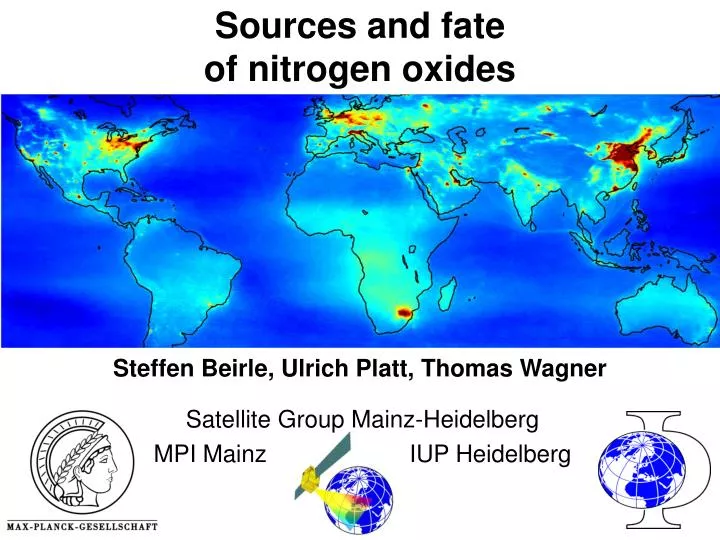
Sources and fate of nitrogen oxides. Satellite Group Mainz-Heidelberg MPI Mainz IUP Heidelberg. Steffen Beirle, Ulrich Platt, Thomas Wagner. Sources and fate of nitrogen oxides. almost. Keep. Everything has been said. Thank you for your attention.

E N D
Sources and fate of nitrogen oxides Satellite Group Mainz-Heidelberg MPI Mainz IUP Heidelberg Steffen Beirle, Ulrich Platt, Thomas Wagner
Sources and fate of nitrogen oxides almost Keep Everything has been said. Thank you for your attention.
Tropospheric NO2: The global picture • For the first time ever! • Meanwhile: >10 years, 4 satellite instruments • Spatial resolution much better than global CTM/GCMs
Tropospheric NO2: What can we learn? • Check our understanding on emissions and chemistry of nitrogen oxides: • Where are the sources? • What is the strength of the different NOx sources? • Trends • Transport and deposition of NOx Chemistry!
Tropospheric NO2: Restrictions • Stratospheric estimation • Sensitivity, AMF • Albedo • Profile • Clouds & Aerosols • Fixed local time • Limited spatial resolution
Tropospheric NO2: How to use? • Comparisons/combinations with (inverse) models • Loss of spatial and temporal resolution • Resulting product: Model or measurement? Gain as much info as possible from the meas.
Tropospheric NO2: What will I talk about • Present some studies on • Source identification & quantification • Estimating lifetimes • This is a workshop: • Some questions ?
NO2 TSCD [1015 molec/cm²] Sources of NOx Fossil fuel comb. 22 (13-31) Biomass burning 8 (3-15) Lightning 5 (2-20) Soil emissions 7 (4-12) Tg [N]/year (Lee et al. 1997) Mean tropospheric slant column density (TSCD) (SCIAMACHY 2003-now)
Fossil fuel combustion • >50% • „Stationary“ sources (transport on prescribed tracks) Constant spatial patterns • Cities • Power plants • Highways? • Ship tracks • Characteristic temporal patterns: • Seasonal variations • Holidays, temporal regulations → Wang et al., 2007 • Weekly cycle!
Fossil fuel combustion: Ship emissions • High uncertainties: 3-7 Tg [N]/yr • Up to 1/3 of total NOx emissions from combustion! • Strong impact: low background NOx • Probably strong increase during next decades AMVER Ship traffic distribution (% of total)
Fossil fuel combustion: Ship emissions • Estimated NOx emissions based on AMVER (Endresen et al., 2003) • b) NO2 TVCD GOME • (Spring, Cloud free) • c) Meridional high-pass filtered TVCD 1013molec/cm2 Beirle et al., 2004 → Richter et al., 2004
Fossil fuel combustion: Ship emissions AMVER ship traffic density (% of total) SCIAMACHY NO2 2003-2004 mean, Land masses masked
Fossil fuel combustion: Ship emissions AMVER ship traffic density (% of total) SCIAMACHY NO2 2003-2006 mean, 2D Highpass-filtered Land masses masked
Fossil fuel combustion: Ship emissions • Future: • Better statistics, increasing ship emissions more & clearer ship tracks • Interaction of ship emissions and sensitivity due to aerosols and clouds??? • Check: 1+1=2? • Gaps??? SCIAMACHY NO2 2003-2006 mean, 2D Highpass-filtered Land masses masked
Fossil fuel combustion: Ship emissions ? Eyring et al. 2007
Fossil fuel combustion: Weekly cycle Europe US Eastcoast Tropospheric NO2 mean vertical column density (GOME, 1996-2001) Beirle et al., 2003
Fossil fuel combustion: Weekly cycle Normalized weekly cycles of NO2 for different parts of the world
Fossil fuel combustion: Trends • China: strong increase Richter et al., 2005 → Van der A et al., 2006
1996-2001 (GOME) 320x40km2 1996-2001 (GOME NSM) 80x40km2 2003-2004 (SCIAMACHY) 60x30km2 Fossil fuel combustion: Trends • Narrow Swath: use GOME high resolution to reconstruct past spatial distribution! → Beirle et al., Highly resolved global distribution of tropospheric NO2 using GOME narrow swath mode data,Atmos. Chem. Phys., 4, 2004.
South America North Africa Central Africa Indonesia Eastern Russia Northern Australia 1998 1999 2000 ATSR fires and GOME NO2 in South-East Asia Biomass burning • Characteristics: • Seasonality • Indicator: Fire counts • Problems: • Saturation • Aerosols! • Profiles! • Lifetime! • Different emission factors → Thomas et al., 1998 →Spichtinger et al., 2004 Very difficult to get quantitative!
Soil emissions • Triggered by rain → Strong temporal fluctuations → Jaegle et al., 2004 → Ron
Lightning • Importance: • UT: low background, long lifetime • Strong impact on UT ozone • High uncertainties! • Characteristics: • Seasonality • Max. over tropical land masses • Specific problems: • Profile? • UT: low NO2/NOx • Clouds
above: flashes [1/day/pixel] below: trop. NO2 [1015 molec/cm2] Lightning • Correlation of lightning and NO2 Correlation of monthly mean flashes (LIS) and NO2 (GOME) for Australia 2.8 (0.8-14) Tg[N]/yr → Beirle et al., Adv. Space Res., 34 (4), 2004.
Lightning Boersma et al., 2005: Correlation of GOME NO2 and TM3 LNO2: 1.1-6.4 Tg [N]/yr
Lightning Martin et al., 2007: Comparison of SCIA NO2 GEOS-Chem: 4-8 Tg [N]/yr
Lightning Unresolved issues: Lightning parameterizations don‘t match Congo maximum! Global Lightning Apr 1995-Feb 2003 LIS / OTD (NASA) flashes/day/km2 • Central Africa: • Highest flash rate globally • 15% of global flashes • →15% of global LNOx production
Lightning • Upper bound: Don‘t care (too much) about biomass burning... • Rough estimate of LNOx: • cloud free: <1.7 Tg N/yr (same assumptions as for Australia case study) • extrapolation not critical: 15% of global flashes! Lightning Biomass burning Winter Summer
Lightning • Upper bound: Don‘t care (too much) about biomass burning... • Rough estimate of LNOx: cloud free, same assumptions as for Australia case study <1.7 Tg [N]/yr
Lightning: Direct observation of fresh LNOx • Conversion factor depends on box AMF and NO2 profile, i.e. LNOx profile and NOx partitioning: ai: Box Air Mass Factor (AMF) pi: normalized NOx profile li: NOx partitioning L = [NO2]/ [NOx]
LNOx profile: Cloud resolving models Pickering et al. 1998 Fehr et al. 2004 NOx partitioning: In-situ measurements in New Mexico for cb conditions Ridley et al. 1994, 1996 Box AMFs: (sensitivity) RTM, cb conditions Hild et al. 2002 [NO2]/[NOx] Box AMF fraction of total ... = 4.02 (2.12-7.14)
Lightning: Direct observation of fresh LNOx • 4 years of SCIAMACHY data • 3 years of WWLLN data (global continuous ground based lightning counts) • Automated search for „lightning events“ prior SCIAMACHY overpass: • grid WWLLN flash counts 5-10 local time on1°x1° grid • mask pixels with >20 flashes („lightning pixel“) • identify clusters of connected lightning pixels with more than 200 flashes in total • keeping lightning clusters that are (partly) covered by SCIAMACHY • 1680 matches!!!
Lightning SCIAMACHY NO2 for WWLLN lightning events 2004-2006 • local time 10 a.m. almost all over ocean • high fluctuations (logarithmic scale) • low NO2 signal
Lightning: Direct observation of fresh LNOx • What is different??? ? 1 10 100 1000
1 10 100 1000 Lightning: Direct observation of fresh LNOx • What is different??? ?
Lightning • What is the reason for the high variability in NO2? • No dependency of NO2 on • Flash counts • CTH • Flash time • Regional differences!? • Where is the LNOx? • Gulf of Mexico case study: LNOx production at lower end! • observed NO2 enhancement 1.6*1015 molec/cm2 • expected: 2.5*1016 molec/cm2 (250 mol per flash, conversion as in the Gulf of Mexico case study) ? ?
Lightning Estimates of LNOx from UV/vis sats • 2.8 (0.8-14) Beirle et al., 2004 • 1.9 (0.5-9.5) Beirle et al., 2004 with updated global flash rate • 1.1-6.4 Boersma et al., 2005 • 1.7 (0.6-4.7) Beirle et al., 2006 • 4-8 Martin et al., 2007 • <1.7 Congo cloud free • ??? Direct SCIAMACHY obs. → What‘s wrong? ?
Transport … • BL: short lifetime of NOx, moderate wind speeds • Annual mean NO2 distribution reflects emissions • Events of medium/longrange transports also happen • Wenig et al., • Stohl et al., • Talk by Mijling
… and lifetime • Transport is determined by wind and lifetime empirical analysis of transport holds information on lifetime • Lifetime: • Hard to measure • Models: nonlinearity, coarse spatial resolution! • Necessary to estimate emissions from NO2 columns
Lifetime: Simple estimates Leue et al., 2001: Mean lifetime ~ 24 hours • Problems: • Multiple, extended sources • GOME pixel width (decrease in SCIAMACHY much steeper) • lifetime overestimated! • Mean(NO2*wind) != mean(NO2)*mean(wind)
Lifetime: Simple estimates Prudhoe Bay Fit: t=4.2 h – at 70°N! 1014 molec/cm2 SCIAMACHY mean, summer
Lifetime: Simple estimates • Ship tracks: (Beirle et al., 2004) • Winds relatively stable • North-South: good GOME resolution • Remaining uncertainty due to daily variation of tau Lifetime estimation: 2.3 hours (summer) 5.1 hours (winter)
Lifetime: Advanced estimates • Model transport: FLEXPART • Consider a point source: Riad • Model spatial patterns for different lifetimes
Lifetime: Advanced estimates Normalized sections of constant longitude (46° E) crossing Riad
Using wind data General additive model: Dependency of NO2 TSCD on Wind direction Preliminary GOME-data 1996-2000, ECMWF wind data M. Hayn, satellite Group Mainz-Heidelberg
Using wind data • NO2-plumes can be followed across the ocean • determination of „influence zone“ Preliminary GOME-data 1996-2000, ECMWF wind data M. Hayn, satellite Group Mainz-Heidelberg
Using wind data: „Fluxes“ • „Flux“ of NO2: Mean(NO2*wind) • Quantify transport • Ocean fertilization • Lifetime Preliminary GOME-data 1996-2000, ECMWF wind data M. Hayn, satellite Group Mainz-Heidelberg
Using wind data: „Fluxes“ Preliminary GOME-data 1996-2000, ECMWF wind data M. Hayn, satellite Group Mainz-Heidelberg
Lifetime: Weekly cycle again... Normalized seazonal weekly cycles of NO2 for Germany → Beirle et al., Weekly cycle of NO2, ACP 3, 2225-2232, 2003.
Spring Summer Autumn Winter Germany 16.1 5.5 15.5 24.2 Po valley 11.2 8.8 12.6 11.3 US Eastcoast 11.6 11.2 23.8 33.2 LA 10.8 6.4 18.2 25.9 Japan 16.0 11.9 24.0 22.1 Lifetime: Weekly cycle again... Lifetime Measured lifetime, independent on models → Beirle et al., Weekly cycle of NO2, ACP 3, 2225-2232, 2003.