Download
1 / 39
390 likes | 514 Views
This document discusses the problem of modernizing roads between cities, represented as a connected, undirected graph. The aim is to create a Minimum Spanning Tree (MST) to connect all cities while minimizing the total modernization cost. Various properties of trees are explored, including acyclicity, edge properties, and the uniqueness of paths. The text outlines algorithms for growing the MST, including Prim's and Kruskal's methods, demonstrating how to identify safe edges for inclusion. This study provides insights into solving graph-based optimization problems effectively.

E N D
Finding Minimum Spanning Trees [CLRS] – Chap 23
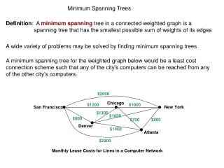
Starting Problem • We have a map of n cities, connected by roads which are in poor condition. For each road, the cost needed for its modernization is known. Create a plan to modernize a subset of all roads, such that any two cities are connected by it and the total cost of the modernization is minimal.
The problem in general terms The problem: Given a connected, undirected graph G=(V;E), and for each edge (u,v) in E, we have a weight w(u,v) specifying the cost to connect u and v. We then want to find a subset T included in E that connects all of the vertices and whose total weight is minimized. We denote: Number of vertexes = n = card(V) = |V| Number of edges = m = card(E)=|E| For a connected, undirected graph: |V| ≤ |E| ≤ |V|2
A very brute force solution • Backtracking • Try to generate all subsets T of edges that connect all V nodes, search the one with total minimum cost • Combinations of |E| taken as |V| • No !!! Can we have a better solution ?
Solution starting points • Question: Has the subgraph (V,T) any interesting properties (that could help us in the search for a solution to this problem) ? • As a first step in finding the solution, we will find and prove such properties
Properties Property 1:If T is the subset of E that connects all of the vertices and whose total weight is minimized, then the graph A=(V,T) is acyclic. Proof: if we suppose that A is not acyclic, but it has a cycle: we could remove an edge from the cycle, the vertexes remain connected but the total weight is reduced => T was not the subset of minimum total weight
Definitions: Graph, Tree, Forest A tree is a connected, acyclic, undirected graph. A forest is a disconnected, acyclic, undirected graph. Definition: the subgraph A is called the Minimum-cost Spanning Tree (MST) of graph G=(V,E)
Tree properties Property 2: The number of edges in a tree T is equal with the number of vertices minus 1. card(T)=card(V)-1 Proof: T is an undirected, acyclic, connected graph. Proof results immediately by induction …
Tree properties Property 3: There is exactly one path between any two nodes of a tree T. Proof: T is an undirected, acyclic, connected graph. Proof results immediately by reductio ad absurdum …
General solution: Growing a MST • We try growing the MST by adding one edge at a time. We will build a set of edges A, which is, at every moment, a subset of a MST. • Loop invariant: Prior to each iteration, A is a subset of some minimum spanning tree. • At each step, we determine a safe edge (u,v) that we can add to A without violating this invariant, in the sense that A plus (u,v) is also a subset of a minimum spanning tree.
General algorithm for growing a MST GENERIC-MST 1 A = {}; 2 while A does not form a spanning tree 3 find an edge (u,v) that is safe for A 4 A = A + (u,v) 5 return A • Crucial question: How do we find the safe edge needed in line 3 ?
Approaches for growing A • A grows as a single tree Loop invariant: Prior to each iteration, A is a subtree of some minimum spanning tree. (Prim’s algorithm) • A can start as a forest of trees. Loop invariant: Prior to each iteration, A is a subset of some minimum spanning tree. (Kruskal’s algorithm)
Building a MST by growing it as a single tree • Loop invariant:Prior to each iteration, A is a subtree of some minimum spanning tree. • Induction hypothesis: Given a graph, we know how to find a subgraph A with k edges, so that A is a subtree of a MST. Ek= the set of all edges connecting nodes in A (denoted as the set AV) with nodes of G that are not yet in A (they are in V-AV). The safe edge = the edge of Ek with the minimum weight. We have to prove that adding the safe edge leads to a subtree of the MST containing k+1 edges.
Building a MST by growing it as a single tree - Example [CLRS – Fig 23.5]
Building a MST by growing it as a single tree - Proof Induction hypothesis: Given a graph, we know how to find a subgraph A with k edges, so that A is a subtree of a MST. We also know (see the tree property 3 presented before), that if A has k edges then it has k+1 nodes. Initialization: • K=0: 1 random start node, 0 edges • K=1: choose the edge with the minimum weight adjacent to the start node. 2 nodes, 1 edge
Building a MST by growing it as a single tree - Proof Maintenance: • K: suppose A is a subtree of the MST, with k edges. The nodes of A form the set AV. • (u,v)= the minimum cost edge from Ek. • We try to suppose that (u,v) does not belong to MST. • In the MST there is a unique path between u and v. Since u is in AV and v is not in AV, this path will contain an edge (x,y) such that x is in AV and y is not in AV. cost(u,v)<cost(x,y), because (u,v) is the minimum from Ek . If we remove (x,y) from the MST and put (u,v), we obtain another spanning tree, with a smaller cost => the spanning tree containing (u,v) is the MST • => by adding (u,v) we got a subtree of the MST with k+1 edges
Building a MST by growing it as a single tree - Proof x y u v u Set of vertexes AV Set of vertexes V- AV
Building a MST by growing it as a single tree - Proof Termination: • Each iteration adds an edge to A • After |V|-1 iterations all the |V| vertexes are connected, A is the MST of graph G
Prim’s algorithm Given G = (V, E). Output: a MST A. Randomly select a vertex v AV = {v}; A = {}. While (AV != V) (X) find a vertex u V-AV that connects to a vertex v AV such that w(u, v) ≤ w(x, y), for any x V-AV and y AV AV = AV U {u}; A = A U (u, v). EndWhile Return A
Comments on Prim’s algorithm • It is a greedy algorithm (it selects the local-best item at every step) • As opposed to typical greedy algorithms that provide approximate results, Prim’s algorithm could be proved that it always finds a minimum cost spanning tree !
Time complexity The while loop has |V| iterations Given G = (V, E). Output: a MST A. Randomly select a vertex v AV = {v}; A = {}. While (AV != V) (X) find a vertex u V-AV that connects to a vertex v AV such that w(u, v) ≤ w(x, y), for any x V-AV and y AV AV = AV U {u}; A = A U (u, v). EndWhile Return A The running time of the algorithm is |V| multiplied with the running time of the operation (X)
Efficient implementation of Prim’s algorithm ? • The efficiency of the algorithm is determined by the efficiency of the operation denoted by (X)– finding the minimum cost edge (u,v) that unites a vertex v already in the MST (in AV) with a vertex u outside it (V-AV) • Possible solutions to this problem: • Brute force: test all edges • Improved: keep the list of vertex candidates in an array • Better: keep vertex candidates in a priority queue
1. Finding (u,v) – Brute force (X)find a vertex u V-AV that connects to a vertex v AV such that w(u, v) ≤ w(x, y), for any x V-AV and y AV min_weight = infinity. For each edge (x, y) in E if x V-AV, y AV, and w(x, y) < min_weight u = x; v = y; min_weight = w(x, y); (X) • time spent per (X) : Θ(|E|) • Total time complexity of MST algo: Θ(|V|*|E|) • Note that |V| ≤ |E| ≤ |V|2 => MST algo is O(|V|3)
2 Finding (u,v) - Distance array • In the case when the number of edges is big - near to |V|2, the brute force approach is not efficient • Improvement idea: instead of iterating through E in search of the minimum edge, iterate through V in search of the vertex that fulfills the condition. • BUT: we must be able to test the condition in O(1) ! • Results that: additional data structures are needed to keep for each vertex v the minimum distance from it to any node already in the set of tree nodes AV. • For each vertex v: • d[v] is the min distance from v to any node already in AV • p[v] is the parent node of v in the spanning tree AV
Prim’s algorithm – with distance array Given G = (V, E). Output: a MST A. For all v V d[v] = infinity; p[v] = null; Randomly select a vertex v AV = {v}; A = {}; d[v]=0; While (AV != V) Search d to find u with the smallest d[u] > 0. AV = AV U {u}; A = A U (u, p[u]). d[u] = 0. For each v in adj[u] if d[v] > w(u, v) d[v] = w(u, v); p[v] = u; EndWhile Return A
Time complexity Given G = (V, E). Output: a MST A. For all v V d[v] = infinity; p[v] = null; Randomly select a vertex v AV = {v}; A = {}; d[v]=0; While (AV != V) Search d to find u with the smallest d[u] > 0. AV = AV U {u}; A = A U (u, p[u]). d[u] = 0. For each v in adj[u] if d[v] > w(u, v) d[v] = w(u, v); p[v] = u; EndWhile Return A The while loop has |V| iterations Θ(|V|) The loop has maximum |V| iterations • Total time complexity of MST algo: Θ(|V| *|V|)
3 Finding (u,v) - priority queue • Searching the nearest vertex takes O(|V|) time with distance array • Improvement: Use a Priority Queue • During execution of the algorithm, all vertices that are not in the tree reside in a min-priority queue Q based on a key attribute. For each vertex , the attribute key is the minimum weight of any edge connecting to a vertex in the tree; • Priority queue operations: • InitPriorityQueue • ExtractMin • ChangeKey • The running time of Prim’s algorithm depends on how we implement the min-priority queue Q !
Complete Prim’s Algorithm MST-Prim(G, w, r) Q = G.V; for each u Q key[u] = ; p[u] = null; key[r] = 0; while (Q not empty) u = ExtractMin(Q); for each v G.Adj[u] if (v Q and w(u,v) < key[v]) p[v] = u; DecreaseKey(v, w(u,v)); The running time of Prim’s algorithm depends on how we implement the min-priority queue Q !
Implementing min-priority queues • Review: Binary Min-Heaps • A heap is a partial ordered binary tree represented as an array, whose elements satisfy the heap conditions • As consequence, the highest priority key is always situated on the first position of the array which materializes the heap.
Binary Min-Heaps 1 1 Heap conditions : ROOT=1 PARENT (i) = i/2 LEFT (i) = 2*i RIGHT (i) = 2*i+1 2 3 2 9 4 6 5 7 3 4 10 11 MIN-HEAP condition : A[PARENT(i)] <= A[i] 8 9 10 5 6 8 1 2 3 4 5 6 7 8 9 10 1 2 9 3 4 10 11 5 6 8
Heap - ExtractMin 1 1 N = number of nodes in heap ExtractMin: Θ(log N) 2 3 2 9 4 6 5 7 3 4 10 11 8 9 10 5 6 8 1 2 3 4 5 6 7 8 9 10 1 2 9 3 4 10 11 5 6 8
Heap - DecreaseKey 1 1 N = number of nodes in heap DecreaseKey: Θ(log N) 2 3 2 9 4 6 5 7 3 4 10 11 8 9 10 5 6 8 1 2 3 4 5 6 7 8 9 10 0 1 2 9 3 4 10 11 5 6 8
Complexity of Prim’s Algorithm MST-Prim(G, w, r) Q = V[G]; for each u Q key[u] = ; p[u] = null; key[r] = 0; while (Q not empty) u = ExtractMin(Q); for each v Adj[u] if (v Q and w(u,v) < key[v]) p[v] = u; DecreaseKey(v, w(u,v)); O(V) Θ(log V) O(V) Θ(log V) Q = a Priority queue based on Heaps A first rough estimation is O(V*log V+V*V*log V) -> but we can calculate more precise !
Complexity of Prim’s Algorithm • ExtractMin gets called exactly once for every vertex -> contributes O(V*log V) • DecreaseKey gets called overall 2*E times -> contributes O(E*log V) • Complexity of Prim’s algorithm when using a priority queue implemented with heaps O(V*log V+ E* log V) = O(E*log V)
Final Performance Analysis • MST algorithm using distance array • O( V* V) • Prim’s algorithm using priority queue based on Heaps • O(E * log V) • For every graph, V<=E<=V*V • Sparse graph: E≈V • Dense graph: E≈V*V => Good for dense graphs => Good for sparse graphs
1 2 3 4 1 1 0 5 6 0 5 2 5 0 9 0 6 2 4 3 6 9 0 4 9 4 3 4 0 0 4 0 Graph representations • Weighted, undirected graph Adjacency Matrix 1 2,5 3,6 Adjacency Lists 2 1,5 3,9 3 1,6 2,9 4,4 4 3,4
Influence of graph representations on MST algorithms • Prim’s algorithm using priority queue based on Heaps should not use adjacency matrixes for graph representation, otherwise it becomes O(V*V*log V) !
Conclusions • Steps for solving algorithmic problems • Identify the abstract model behind the problem story. Make clear what we are looking for • Identify and prove properties of the solution that may be helpful in finding it • Design the algorithm “in the large” (without worrying about low-level implementation details), prove it • Refine the details of the algorithm, search for solutions to reduce complexity • Decide the final implementation details
What we learned today • Steps for solving algorithmic problems • Minimum Spanning Trees. Prim’s algorithm [CLRS chap 23] • Review: Heaps. Priority Queues [CLRS chap 6]