Download
1 / 28
280 likes | 500 Views
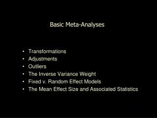
Basic Meta-Analyses. Transformations Adjustments Outliers The Inverse Variance Weight Fixed v. Random Effect Models The Mean Effect Size and Associated Statistics. Transformations.

E N D
Basic Meta-Analyses • Transformations • Adjustments • Outliers • The Inverse Variance Weight • Fixed v. Random Effect Models • The Mean Effect Size and Associated Statistics
Transformations The most basic meta analysis is to take the average of the effect size from multiple studies as the best estimate of the effect size of the population of studies of that effect. As you know, taking the average of a set of values “works better” if the values are normally distributed! In order to ask if that mean effect size is different from 0, we’ll have to compute a standard error of the estimated mean, and perform a Z-test. The common formulas for both of these also “work better” if the effect sizes are normally distributed. And therein lies a problem! None of d, r & odds ratios are normally distributed!!! So, it is a good idea to transform the data before performing these calculations !!
Transformations -- d d has an upward bias when sample sizes are small • the extent of bias depends upon sample size • the result is that a set of d values (especially with different sample sizes) isn’t normally distributed • a correction for this upward bias & consequent non-normality is available 3 ES = d * 1 - -------- 4N-9 Excel formula is d * ( 1 - (3 / ((4*N) – 9)))
Transformations -- r r is not normally distributed • and it has a problematic standard error formula. • Fisher’s Zr transformation is used – resulting in a set of ES values that are normally distributed 1 + r ES = .5 * ln ------- 1 - r Excel formula is FISHER(r) • all the calculations are then performed using the ES • the final estimate of the population ES can be returned to r using another formula (don’t forget this step!!!) e 2ES - 1 r = ------------ e 2ES + 1 Excel formula is FISHERINV(ES)
Transformations – Odds-Ratio the OR is asymmetrically distributed • and has a complex standard error formula. • one solution is to use the natural log of the OR • nice consequence is that the transformed values are interpreted like d & r • Negative relationship < 0. • No relationship = 0. • Positive relationship > 0. Excel formula is LN(OR) ES = ln [OR] • all the calculations are then performed using the ES • the final estimate of the population ES can be returned to OR using another formula (don’t forget this step!!!) OR = e ES Excel formula is EXP(ES)
Adjustments(less universally accepted than transformations!!) r r’ = ------- DV measurement unreliability • what would r be if the DV were perfectly reliable? • need reliability of DV () • range restriction • What would r be if sample had full range of population DV scores ? • “s” is sample std • need unrestricted population std (“S”) S*r r’ = ----------------------- (S2r2 + s2 – s2r2) Can use r d formulas to obtain these
Adjustments, cont.(less universally accepted than transformations!!) • artificial dichotomization of measures • What would effect size be if variables had been measured as quantitative? • If DV was dichotomized • e.g., Tx-Cx & pass-fail instead of % correct • use biserial correlation • If both variables dichotomized • e.g., some-none practices & pass-fail, instead of #practices & % correct • Use tetrachoric correlation
Adjustments, cont.(less universally accepted than transformations!!) Outliers • As in any aggregation, extreme values may have disproportionate influence • Identification using Mosteller & Tukey method is fairly common • Trimming and Winsorizing are both common For all adjustments – Be sure to tell your readers what you did & the values you used for the adjustments!
The Inverse Variance Weight • An ES based on 400 participants is assumed to be a “better” estimate of the population ES than one based on 50 participants. • So, ESs from larger studies should “count for more” than ESs from smaller studies! • Original idea was to weight each ES by its sample size. • Hedges suggested an alternative… • we want to increase the precision of our ES estimates • he showed that weighting ESs by their inverse variance minimizes the variance of their sum (and mean), and so, minimizes the Standard Error (SE) • the resulting smaller Standard Error leads to narrower CIs and more power full significance tests!!! • The optimal weight is 1 / SE2
Calculating Inverse Variance Weights for Different Effect Sizes d*** r*** Odds Ratio*** ***Note:Applied to ESs that have been transformed to normal distn
Weighted Mean Effect Size The most basic “meta analysis” is to find the average ES of the studies chose to represent the population of studies of “the effect”. The formula is pretty simple – the sum of the weighted ESs, divided by the sum of the weightings. • But much has happened to get to here! • select & obtain studies to include in meta analyis • code study for important attributes • extract d, dgain, r, OR • ND transformation of d, r, or OR • perhaps adjust for unreliability, range restriction or outliers • Note: we’re about to assume there is a single population of studies represented & that all have the same effect size, except for sampling error !!!!!
Weighted Mean Effect Size One more thing… Fixed Effects vs. Random Effects Meta Analysis Alternative ways of computing and testing the mean effect sizes. Which you use depends on…. How you conceptualize the source(s) of variation among the study effect sizes – why don’t all the studies have the same effect size??? And leads to …How you will compute the estimate and the error of estimate. Which influences… The statistical results you get!
Fixed Effect Models • Assume each study in the meta-analysis used the same (fixed) operationalizations of the design conditions & same external validity elements (population, setting, task/stimulus) • (Some say they also assume that the IV in each study is manipulated (fixed), so the IV in every study is identical.) • Based on this, the studies in the meta analysis are assumed to be drawn from a population of studies that all have the same effect size, except for sampling error • So, the sampling error is inversely related to the size of the sample • which is why the effect size of each study is weighted by the inverse variance weight (which is computed from sample size)
Random Effect Models • Assume different studies in the meta-analysis used different operationalizations of the design conditions, and/or different external validity elements (population, setting, task/stimulus) • Based on this, studies in the meta analysis are assumed to be drawn from a population of studies that have different effect sizes for two reasons: • Sampling variability • “Real” effect size differences between studies caused by the differences in operationalizations and external validity elements • So, the sampling error is inversely related to the size of the sample and directly related to the variability across the population of studies • Compute the • inverse weight differently
How do you choose between Fixed & Random Effect Models ??? • The assumptions of the Fixed Effect model are less likely to be met than those of the Random Effect model. Even “replications” don’t use all the same external validity elements and operationalizations… • The sampling error estimate of the Random Effect model is likely to be larger, and, so, the resulting statistical tests less powerful than for the Fixed Effect model • It is possible to test to see if the amount of variability (heterogeneity) among a set of effect sizes is larger than would be expected if all the effect sizes came from the same population. Rejecting the null is seen by some as evidence that a Random Effect model should be used. It is very common advice to compute mean effect sizes using both approaches, and to report both sets of results!!!
Computing Fixed Effects weighted mean ES This example will use “r”. Step 1 There is a row or case for each effect size. The study/analysis each effect size was taken from is noted. The raw effect size “r” and sample size (n) is given for each of the effect sizes being analyzed.
Step 2 Use Fisher’s Z transform to normalize each “r” Label the column Highlight a cell Type “=“ and the formula (will appear in the fx bar above the cells) Copy that cell into other cells in that column All further computations will use ES(Zr) Formula is FISHER( “r” cellref )
Step 3 Compute inverse variance weight Label the column Highlight a cell Type “=“ and the formula (will appear in the fx bar above the cells) Copy that cell into other cells in that column Also compute sum of ES Formula is “n” cellref - 3 Rem: the inverse variance weight (w) is computed differently for different types of ES
Step 4 Compute weighted ES Label the column Highlight a cell Type “=“ and the formula (will appear in the fx bar above the cells) Copy that cell into other cells in that column Formula is “ES (Zr)” cellref * “w” cellref
Step 5 Get sums of weights and weighted ES Add the “Totals” label Highlight cells containing “w” values Click the “Σ” Sum of those cells will appear below last cell Repeat to get sum of weighted ES (shown)
Step 6 Compute weighted mean ES Add the label Highlight a cell Type “=“ and the formula (will appear in the fx bar above the cells) “sum weightedES” cellref ----------------------------------- “sum weights” cellref The formula is
Computing weighted mean r Step 7 Transform mean ES r Add the label Highlight a cell Type “=“ and the formula (will appear in the fx bar above the cells) The formula is FISHERINV( “meanES” cellref ) Ta Da !!!!
Z-test of mean ES ( also test of r ) Step 1 Compute Standard Error of mean ES Add the label Highlight a cell Type “=“ and the formula (will appear in the fx bar above the cells) The formula is SQRT(1 / “sum of weights” cellref )
Z-test of mean ES ( also test of r ) Step 2 Compute Z Add the label Highlight a cell Type “=“ and the formula (will appear in the fx bar above the cells) The formula is “weighted Mean ES cellref” / “SE mean ES cellref” Ta Da !!!!
CIs Step 1 Compute CI values for ES Add the labels Highlight a cell Type “=“ and the formula (will appear in the fx bar above the cells) The formulas are Lower “wtdMean ES” cellref – (1.96 * “SE Mean ES” cellref ) Upper “wtdMean ES” cellref + (1.96 * “SE Mean ES” cellref )
CIs Step 2 Convert ES bounds r bounds Add the label Highlight a cell Type “=“ and the formula (will appear in the fx bar above the cells) The formula for each is FISHERINV( “CI boundary” cellref ) Ta Da !!!!
Here are the formulas we’ve used… Mean ES SE of the Mean ES Z-test for the Mean ES 95% Confidence Interval
What about computing a Random Effect weighted mean ES?? It is possible to compute a “w” value that takes into account both the random sampling variability among the studies and the systematic sampling variablity. Then you would redo the analyses using this “w” value – and that would be a Random Effect weighted mean ES! Doing either with a large set of effect sizes, using XLS, is somewhat tedious, and it is easy to make an error that is very hard to find. Instead, find the demo of how to use the SPSS macros written by David Wilson.