Download
1 / 14
150 likes | 437 Views
Chapter 5 Initial-Value Problems for Ordinary Differential Equations -- Euler’s Method. Compute the approximations of y ( t ) at a set of ( usually equally-spaced ) mesh points a = t 0 < t 1 <…< t n = b . That is, to compute w i y ( t i ) = y i for i = 1, …, n.

E N D
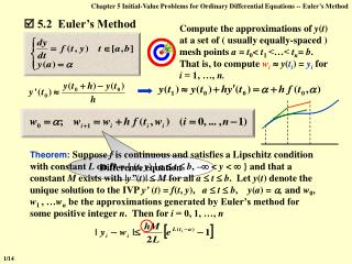
Chapter 5 Initial-Value Problems for Ordinary Differential Equations -- Euler’s Method Compute the approximations of y(t) at a set of ( usually equally-spaced ) mesh points a = t0< t1 <…< tn= b. That is, to compute wi y(ti) = yi for i = 1, …, n. 5.2 Euler’s Method Theorem: Suppose f is continuous and satisfies a Lipschitz condition with constant L on D = { (t, y) | a t b, – < y < } and that a constant M exists with |y”(t)| M for all a t b. Let y(t) denote the unique solution to the IVP y’ (t) = f(t, y), a t b, y(a) = , and w0, w1 , …wn be the approximations generated by Euler’s method for some positive integer n. Then for i = 0, 1, …, n Difference equation 1/14
Chapter 5 Initial-Value Problems for Ordinary Differential Equations -- Euler’s Method + 0 + i+1 Note: y”(t) can be computed without explicitly knowing y(t). The roundoff error Theorem: Let y(t) denote the unique solution to the IVP y’ (t) = f(t, y), a t b, y(a) = , and w0, w1 , …wn be the approximations obtained using the above difference equations. If | i | < for i = 0, 1, …, n, then for each i 2/14
Chapter 5 Initial-Value Problems for Ordinary Differential Equations -- Higher Order Taylor Methods Definition: The difference method w0 = ; wi+1 = wi + h( ti, wi), for each i = 0, 1, …, n – 1 has local truncation error for each i = 0, 1, …, n – 1. 5.3 Higher Order Taylor Methods Note: The local truncation error is just (yi+1wi+1)/h with the assumption that wi=yi. The local truncation error of Euler’s method Method of order 1 3/14
Chapter 5 Initial-Value Problems for Ordinary Differential Equations -- Higher Order Taylor Methods Taylor method of order n: where Note: Euler’s method can be derived by using Taylor’s expansion with n = 1 to approximate y(t). Higher Order Taylor Methods The local truncation error is O(hn) if y Cn+1[a, b]. 4/14
Chapter 5 Initial-Value Problems for Ordinary Differential Equations -- Higher Order Taylor Methods T (2)(ti, wi) = Taylor’s method of order 2: Example: Apply Taylor’s method of order 2 and 4 to the IVP y’ = y – t2 + 1, 0 t 2, y(0) = 0.5 Solution: Find the first 3 derivatives of f f(t, y(t)) = y(t) – t2 + 1 HW: p.271 #5 (a)(b) f ’(t, y(t)) = y’(t) – 2t = y(t) – t2 + 1 – 2t f ”(t, y(t)) = y’(t) – 2t – 2 = y(t) – t2– 2t – 1 f (3)(t, y(t)) = y’(t) – 2t – 2 = y(t) – t2– 2t – 1 Given n = 10, then h = 0.2 and ti = 0.2i Table 5.3 on p.269 wi+1 = 1.22wi – 0.0088i2– 0.008i + 0.22 5/14
Chapter 5 Initial-Value Problems for Ordinary Differential Equations -- Higher Order Taylor Methods + = a + y ( t ) y ( t ) h y’ ( t ) h f ( t , y ( t )) 1 0 1 1 1 = a = + = - w ; w w h f ( t , w ) ( i 0 , ... , n 1 ) + + + 0 1 1 1 i i i i Hey! Isn’t the local truncation error of Euler’s method ? Seems that we can make a good use of it … Other Euler’s Methods Implicit Euler’s method Usually wi+1 has to be solved iteratively, with an initial value given by the explicit method. The local truncation error of the implicit Euler’s method 6/14
Chapter 5 Initial-Value Problems for Ordinary Differential Equations -- Higher Order Taylor Methods Trapezoidal Method Two initial points are required to start moving forward. Such a method is called double-step method. All the previously discussed methods are single-step methods. Note: The local truncation error is indeed O(h2). However an implicit equation has to be solved iteratively. Double-step Method Note: If we assume that wi – 1=yi– 1and wi=yi, the local truncation error is O(h2). 7/14
Chapter 5 Initial-Value Problems for Ordinary Differential Equations -- Higher Order Taylor Methods Method Euler’s explicit Euler’s implicit Trapezoidal Double-step Simple Low order accuracy stable Low order accuracy and time consuming More accurate Time consuming More accurate, and explicit Requires one extra initial point Can’t you give me a method with all the advantages yet without any of the disadvantages? Do you think it possible? Well, call me greedy… OK, let’s make it possible. 8/14
Chapter 5 Initial-Value Problems for Ordinary Differential Equations -- Higher Order Taylor Methods Step 1:Predict a solution by the explicit Euler’s method = + w w h f ( t , w ) + 1 i i i i Step 2: Correctwi+1 by Plugging it into the right hand side of the trapezoidal formula h = + + w w [ f ( t , w ) f ( t , w )] + + + 1 1 1 i i i i i i 2 Modified Euler’s Method Note: This kind of method is called the predictor-corrector method. This modified Euler’ method is a single-step method of order 2. It is simpler than the implicit methods and is more stable that the explicit Euler’s method. 9/14
Chapter 5 Initial-Value Problems for Ordinary Differential Equations -- Runge-Kutta Methods A single-step method with high-order local truncation error without evaluating the derivatives of f. In a single-step method, a line segment is extended from (ti, wi) to reach the next point (ti+1, wi +1) according to some slope. We can improve the result by finding a better slope. Idea 5.4 Runge-Kutta Methods Must the slope be the average of K1and K2 ? Check the modified Euler’s method: Must the step size be h? 10/14
Chapter 5 Initial-Value Problems for Ordinary Differential Equations -- Runge-Kutta Methods Generalize it to be: = + l + l w w h [ K K ] + 1 1 1 2 2 i i = K f ( t , w ) 1 i i = + + K f ( t ph , w phK ) 2 1 i i Step 2: Plug K2 into the first equation Determine 1, 2, and p such that the method has local truncation error of order 2. Step 1: Write the Taylor expansion of K2at ( ti , yi ) : Step 3: Find 1, 2, and p such thati+1 = ( yi+1 – wi+1 )/h = O(h2). 11/14
Chapter 5 Initial-Value Problems for Ordinary Differential Equations -- Runge-Kutta Methods Here are unknowns and equations. 3 2 There are infinitely many solutions. A family of methods generated from these two equations is called Runge-Kutta method of order 2. Note: The modified Euler’s method is only a special case of Runge-Kutta methods with p = 1 and 1 = 2 = 1/2. Q: How to obtain higher-ordered accuracy? 12/14
Chapter 5 Initial-Value Problems for Ordinary Differential Equations -- Runge-Kutta Methods = + l + l + + l w y h [ K K ... K ] + 1 1 1 2 2 i i m m = K f ( t , w ) 1 i i = + a + b K f ( t h , w hK ) 2 2 21 1 i i = + a + b + b K f ( t h , w hK hK ) 3 3 31 1 32 2 i i ... ... = + a + b + b + + b hK ) K f ( t h , wi hK hK ... - - 1 m 1 1 2 2 1 m i m m m m m Classical Runge-Kutta Order 4 Method – the most popular one 13/14
Chapter 5 Initial-Value Problems for Ordinary Differential Equations -- Runge-Kutta Methods Note: The main computational effort in applying the Runge-Kutta methods is the evaluation of f. Butcher has established the relationship between the number of evaluations per step and the order of the local truncation error : evaluations per step 2 3 4 5-7 8-9 n10 Best possible LTE HW: p.280-281 #1 (a), 10, 13 Since Runge-Kutta methods are based on Taylor’s expansion, y has to be sufficiently smooth to obtain better accuracy with higher-order methods. Usually the methods of lower order are used with smaller step size in preference to the higher-order methods using a large step size. 14/14