Download
1 / 34
340 likes | 345 Views
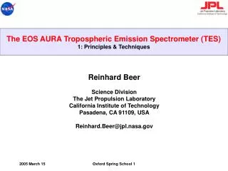
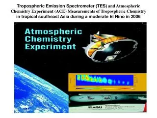
The EOS AURA Tropospheric Emission Spectrometer (TES) 1: Principles & Techniques. Reinhard Beer Science Division The Jet Propulsion Laboratory California Institute of Technology Pasadena, CA 91109, USA Reinhard.Beer@jpl.nasa.gov. Recommended Texts.

E N D
The EOS AURA Tropospheric Emission Spectrometer (TES) 1: Principles & Techniques Reinhard Beer Science Division The Jet Propulsion Laboratory California Institute of Technology Pasadena, CA 91109, USA Reinhard.Beer@jpl.nasa.gov Oxford Spring School 1
Recommended Texts “Remote Sensing by Fourier Transform Spectrometry”, Reinhard Beer, John Wiley & Sons Inc., New York (1992) “The Fast Fourier Transform”, E. Oran Brigham, Prentice-Hall Inc., New Jersey (1974) Both texts are somewhat dated, but still serve as good introductions. Oxford Spring School 1
The TES Experiment Global measurements of tropospheric ozone and its precursors from TES combined with in-situ data and model predictions will address the following key questions: How is the increasing ozone abundance in the troposphere affecting - air quality on a global scale? - oxidizing reactions that “cleanse” the atmosphere? - climate change? Oxford Spring School 1
TES Standard Products N = Nadir, L = Limb Viewing Oxford Spring School 1
The TES Instrument TES is an infrared imaging Fourier Transform Spectrometer (FTS) operating in the spectral range 650 – 3050 cm-1 (roughly 3.3 – 15.4 mm). It features 4 1x16 element optically-conjugated focal plane arrays each optimized for a different spectral region and operating at a temperature of 63K using mechanical refrigerators. In addition, each focal plane is equipped with interchangeable cooled filters that limit the instantaneous spectral bandwidths to about 250 cm-1. This provides needed control over the instrument thermal background and reduces the data rate. Except for two external mirrors (part of the pointing system), the entire optical path is radiatively-cooled to about 165K, further to reduce the instrument background. A particular feature of TES is that it can, unlike any other spaceborne FTS instrument, observe both downwards and sideways to the limb. Oxford Spring School 1
First Principles Oxford Spring School 1
The Principle of Superposition electromagnetic amplitudes are additive Imagine 2 wavetrains of the same amplitude and frequency: Oxford Spring School 1
and Let the wavetrains be Upon addition, we get Setting and dropping the subscripts we end with which represents a wavetrain of the same frequency but phase shifted by D/2 (second cosine term) and an amplitude (first cosine term) that depends on the phase difference. Observe that the resultant amplitude can vary between 2A and zero. Oxford Spring School 1
Spectrometric Units The units most commonly used in spectrometry are the nanometre (1 nm = 10-9 metres), the micrometre (1 mm = 10-6 metres) and the reciprocal centimetre (cm-1). For reasons that will become clear, it is this latter unit that is most commonly used in infrared spectrometry. CONVERSION FACTORS: 1 cm-1 = (Frequency in Hertz)/(Velocity of light) = 107/(wavelength in nanometres) = 104/(wavelength in micrometres) Occasionally, one will see the cm-1 referred to as the wavenumber. This is a description, NOT A UNIT! Oxford Spring School 1
Two-Beam Interference Recall the expression The intensity is therefore Replacing A2 by Iin, the incident intensity of each wavetrain, we get It is evident that I will alternate between 4Iin and 0 as D changes through an amount These two extreme conditions are termed constructive and destructive interference, respectively (although any intermediate condition is equally possible). Oxford Spring School 1
The geometric path difference between beams 1 & 2 is IJ + JK where IJ+JK = d/cos(q) +d.cos(2.q)/cos(q) = 2.d.cos(q) This expression can also be described by a number of wavelengths: nl = 2.d.cos(q). If the interferometer is embedded in a medium of refractive index m, this becomes nl = 2.m.d.cos(q). As stated earlier, we prefer to work in a frequency unit n = 1/l, so, finally, we get n = 2.m.n.d.cos(q) which is the fundamental equation for most types of interferometer. Oxford Spring School 1
Spectral Resolution (1) Spectral Resolution is a measure of the ability of the spectrometer to discriminate between adjacent spectral features. As we shall see, the spectral resolution of a Fourier Transform Spectrometer (henceforth FTS) is inversely proportional to the maximum path difference employed. It must, however, be recognized that improved spectral resolution comes at the price of reduced signal-to-noise ratio, so the maximum path difference employed must be carefully “tuned” to the specific problem to be addressed. In short – enough but not too much! Oxford Spring School 1
Variation of Typical Linewidths with Altitude Oxford Spring School 1
Spectral Resolution (2) Now understanding what is desirable for spectral resolution, how does this apply to an FTS? Remembering an earlier equation for the monochromatic case: we can readily change it (and some notation) for the broad-band case: The first integral is simply the area under the spectrum (i.e., is an additive constant that can be ignored). The second integral will be recognized as the cosine Fourier Transform of Now, Fourier Transforms are defined over infinite ranges in both domains. We overcome the problem in the frequency domain through the use of optical filters. That is, we force outside some range In the path difference (x) domain, it is a different story. Because we can only change path difference (scan) over some finite range Xmax (in either sense, or both), this is mathematically equivalent to multiplying the “infinite” interferogram by a boxcar function that = 1 over the scanned range and is zero elsewhere. Now, a multiplication in interferogram space is identical to a convolution in spectrum space. The Fourier Transform of a boxcar is the well-known “sinc” (= sin[x]/x) function which therefore serves to define the spectral resolution of an ideal FTS. Oxford Spring School 1
Reality Oxford Spring School 1
View of the TES engineering model interferometer retroreflector Oxford Spring School 1
TES Instrumental Line Shape (ILS) Oxford Spring School 1
TES Observation Geometry Oxford Spring School 1
TES Operating Modes Global Survey:16 orbits of nadir & limb observations repeated every other day. This is the source of Standard Products. Stare:Point at a specific latitude & longitude for up to ~4 minutes. Transect:Point at a set of contiguous latitudes & longitudes to cover ~850 km. Step-&-Stare:Point at nadir for 4 seconds (5.2 seconds with necessary reset). Spacecraft has moved ~40 km. Point at nadir again. Repeat indefinitely. Limb Drag: Point at the trailing limb (16 second scans). Repeat indefinitely. These last 4 modes constitute Special Products that are obtained only when no Global Survey is scheduled. Oxford Spring School 1
x x TES Step & Stare, Stare and Transect Modes STEP & STARE: A set of nadir footprints spaced about 35 km apart. Can be indefinite. STARE: Point at a specific latitude & longitude for up to 210 seconds. TRANSECT: A set of exactly contiguous latitudes & longitudes in a line up to 885 km long. Oxford Spring School 1
TES specifications • Fourier transform spectrometer • Wavelength response: 3.3 to 15.4 micron • One scan every 4 or 16 sec. (0.1 cm-1 or 0.025 cm-1 res.) • Four optically-conjugated 1x16 pixel detector arrays • Spatial resolution of 5 x 8 km at nadir & 2.3 km at limb • Passively cooled • 2-axis gimbaled pointing mirror Oxford Spring School 1
TES Limb View Nadir View TES on the Aura Spacecraft Oxford Spring School 1
AURA Launch; 2004 July 15, 03:02 PDT Oxford Spring School 1
Level 1B: Produces radiometrically and frequency calibrated spectra with NESR. Level 2: Produces VMR and temperature profiles. Level 3: Produces global maps. TES Algorithm Overview Level 1A: Produces geolocated interferograms. Oxford Spring School 1
CONCLUSIONS TES is fulfilling its promise to provide the first-ever global overview of the key constituents of tropospheric chemistry and their inter-regional transport For more information: http://tes.jpl.nasa.gov Oxford Spring School 1