Download
1 / 21
210 likes | 414 Views
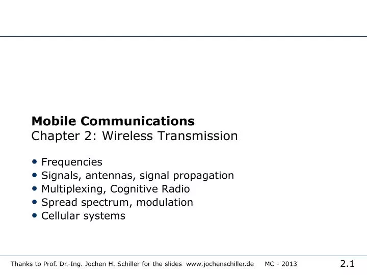
Mobile Communications Chapter 2: Wireless Transmission. Frequencies Signals, antennas, signal propagation Multiplexing, Cognitive Radio Spread spectrum, modulation Cellular systems. Wireless communications. The physical media – Radio Spectrum

E N D
Mobile CommunicationsChapter 2: Wireless Transmission Frequencies Signals, antennas, signal propagation Multiplexing, Cognitive Radio Spread spectrum, modulation Cellular systems Thanks to Prof. Dr.-Ing. Jochen H. Schiller for the slides www.jochenschiller.de MC - 2013
Wireless communications • The physical media – Radio Spectrum • There is one finite range of frequencies over which radio waves can exist – this is the Radio Spectrum • Spectrum is divided into bands for use in different systems, so Wi-Fi uses a different band to GSM, etc. • Spectrum is (mostly) regulated to ensure fair access Thanks to Prof. Dr.-Ing. Jochen H. Schiller for the slides www.jochenschiller.de MC - 2013
Frequencies for communication • VLF = Very Low Frequency UHF = Ultra High Frequency • LF = Low Frequency SHF = Super High Frequency • MF = Medium Frequency EHF = Extra High Frequency • HF = High Frequency UV = Ultraviolet Light • VHF = Very High Frequency • Frequency and wave length • = c/f • wave length , speed of light c 3x10⁸m/s, frequency f twisted pair coax cable optical transmission 1 Mm 300 Hz 10 km 30 kHz 100 m 3 MHz 1 m 300 MHz 10 mm 30 GHz 100 m 3 THz 1 m 300 THz visible light VLF LF MF HF VHF UHF SHF EHF infrared UV Thanks to Prof. Dr.-Ing. Jochen H. Schiller for the slides www.jochenschiller.de MC - 2013
Example frequencies for mobile communication • VHF-/UHF-ranges for mobile radio • simple, small antenna for cars • deterministic propagation characteristics, reliable connections • SHF and higher for directed radio links, satellite communication • small antenna, beam forming • large bandwidth available • Wireless LANs use frequencies in UHF to SHF range • some systems planned up to EHF • limitations due to absorption by water and oxygen molecules (resonance frequencies) • weather dependent fading, signal loss caused by heavy rainfall etc. Thanks to Prof. Dr.-Ing. Jochen H. Schiller for the slides www.jochenschiller.de MC - 2013
Frequencies and regulations • In general: ITU-R holds auctions for new frequencies, manages frequency bands worldwide (WRC, World Radio Conferences) Thanks to Prof. Dr.-Ing. Jochen H. Schiller for the slides www.jochenschiller.de MC - 2013
Signals I • physical representation of data • function of time and location • signal parameters: parameters representing the value of data • classification • continuous time/discrete time • continuous values/discrete values • analog signal = continuous time and continuous values • digital signal = discrete time and discrete values Thanks to Prof. Dr.-Ing. Jochen H. Schiller for the slides www.jochenschiller.de MC - 2013
Signals I • signal parameters of periodic signals: • period T: time to complete a wave. • frequency f=1/T :no of waves generated per second • amplitude A : strength of the signal • phase shift :where the wave starts and stops • sine wave as special periodic signal for a carrier: s(t) = At sin(2 ftt + t) • These factors are transformed into the exactly required signal by Fourier transforms. Thanks to Prof. Dr.-Ing. Jochen H. Schiller for the slides www.jochenschiller.de MC - 2013
Fourier representation of periodic signals 1 1 0 0 t t ideal periodic signal real composition (based on harmonics) • It is easy to isolate/ separate signals with different frequencies using filters Thanks to Prof. Dr.-Ing. Jochen H. Schiller for the slides www.jochenschiller.de MC - 2013
Signals II • Different representations of signals • amplitude (amplitude domain) • frequency spectrum (frequency domain) • phase state diagram (amplitude M and phase in polar coordinates) • Composed signals transferred into frequency domain using Fourier transformation • Digital signals need • infinite frequencies for perfect transmission • modulation with a carrier frequency for transmission (analog signal!) Q = M sin A [V] A [V] t[s] I= M cos f [Hz] Thanks to Prof. Dr.-Ing. Jochen H. Schiller for the slides www.jochenschiller.de MC - 2013
Antennas: isotropic radiator • Radiation and reception of electromagnetic waves, coupling of wires to space for radio transmission • Isotropic radiator: equal radiation in all directions (three dimensional) - only a theoretical reference antenna • Real antennas do not produce radiate signals in equal power in all directions. They always have directive effects (vertically and/or horizontally) • Radiation pattern: measurement of radiation around an antenna z y z ideal isotropic radiator y x x Thanks to Prof. Dr.-Ing. Jochen H. Schiller for the slides www.jochenschiller.de MC - 2013
Antennas: simple dipoles • Real antennas are not isotropic radiators but, e.g., dipoles with lengths /4 on car roofs or /2 as Hertzian dipole shape of antenna proportional to wavelength • Example: Radiation pattern of a simple Hertzian dipole • Omni-Directional Antennas are wasteful in areas where obstacles occur (e.g. valleys) /4 /2 y y z simple dipole x z x side view (xy-plane) side view (yz-plane) top view (xz-plane) Thanks to Prof. Dr.-Ing. Jochen H. Schiller for the slides www.jochenschiller.de MC - 2013
Directional antennas reshape the signal to point towards a target, e.g. an open street • Placing directional antennas together can be used to form cellular reuse patterns • Gain: maximum power in the direction of the main lobe compared to the power of an isotropic radiator (with the same average power) • Often used for microwave connections or base stations for mobile phones (e.g., radio coverage of a valley) • Directed antennas are typically used in cellular systems, several directed antennas combined on a single pole to constructSectorized antennas. Thanks to Prof. Dr.-Ing. Jochen H. Schiller for the slides www.jochenschiller.de MC - 2013
Antennas: directed and sectorized y y z directed antenna x z x side view (xy-plane) side view (yz-plane) top view (xz-plane) z z sectorized antenna x x top view, 3 sector top view, 6 sector Thanks to Prof. Dr.-Ing. Jochen H. Schiller for the slides www.jochenschiller.de MC - 2013
Antennas: diversity • Multi-element antenna arrays: Grouping of 2 or more antennas • multi-element antenna arrays • Antenna diversity • switched diversity, selection diversity • receiver chooses antenna with largest output • diversity combining • combine output power to produce gain • cophasing needed to avoid cancellation /2 /2 /4 /2 /4 /2 + + ground plane Thanks to Prof. Dr.-Ing. Jochen H. Schiller for the slides www.jochenschiller.de MC - 2013
Smart antennas use signal processing software to adapt to conditions –e.g. following a moving receiver (known as beam forming), these are some way off commercially • E.g. wireless devices direct the electro magnetic radiation away from human body toward a base station to reduce the absorbed radiation. Thanks to Prof. Dr.-Ing. Jochen H. Schiller for the slides www.jochenschiller.de MC - 2013
Signal propagation ranges • Transmission range • communication possible • low error rate • Detection range • detection of the signal possible • no communication possible • Interference range • signal may not be detected • signal adds to the background noise • Wireless is less predictable since it has to travel in unpredictable substances – air, dust, rain, bricks sender transmission distance detection interference Thanks to Prof. Dr.-Ing. Jochen H. Schiller for the slides www.jochenschiller.de MC - 2013
Signal propagation: Path loss (attenuation) • In free space signals propagate as light in a straight line (independently of their frequency). • If a straight line exists between a sender and a receiver it is called line-of-sight (LOS) • Receiving power proportional to 1/d² in vacuum (free space loss) – much more in real environments(d = distance between sender and receiver) • Situation becomes worse if there is any matter between sender and receiver especially for long distances • Atmosphere heavily influences satellite transmission • Mobile phone systems are influenced by weather condition as heavy rain which can absorb much of the radiated energy Thanks to Prof. Dr.-Ing. Jochen H. Schiller for the slides www.jochenschiller.de MC - 2013
Signal propagation: Path loss (attenuation) • Radio waves can penetrate objects depending on frequency. The lower the frequency, the better the penetration • Low frequencies perform better in denser materials • High frequencies can get blocked by, e.g. Trees • Radio waves can exhibit three fundamental propagation behaviours depending on their frequencies: • Ground wave (<2 MHz): follow the earth surface and can propagate long distances – submarine communication • Sky wave (2-30 MHz): These short waves are reflected at the ionosphere. Waves can bounce back and forth between the earth surface and the ionosphere, travelling around the world – International broadcast and amateur radio • Line-of-sight (>30 MHz): These waves follow a straight line of sight – mobile phone systems, satellite systems Thanks to Prof. Dr.-Ing. Jochen H. Schiller for the slides www.jochenschiller.de MC - 2013
Signal propagation • Propagation in free space always like light (straight line) • Receiving power proportional to 1/d² in vacuum – much more in real environments, e.g., d3.5…d4(d = distance between sender and receiver) • Receiving power additionally influenced by • fading (frequency dependent) • shadowing • reflection at large obstacles • refraction depending on the density of a medium • scattering at small obstacles • diffraction at edges refraction shadowing reflection scattering diffraction Thanks to Prof. Dr.-Ing. Jochen H. Schiller for the slides www.jochenschiller.de MC - 2013
Multipath propagation • Signal can take many different paths between sender and receiver due to reflection, scattering, diffraction • Time dispersion: signal is dispersed over time • interference with “neighbor” symbols, Inter Symbol Interference (ISI) • The signal reaches a receiver directly and phase shifted • distorted signal depending on the phases of the different parts multipath pulses LOS pulses • LOS • (line-of-sight) signal at sender signal at receiver Thanks to Prof. Dr.-Ing. Jochen H. Schiller for the slides www.jochenschiller.de MC - 2013
Effects of mobility • Channel characteristics change over time and location • signal paths change • different delay variations of different signal parts • different phases of signal parts • quick changes in the power received (short term fading) • Additional changes in • distance to sender • obstacles further away • slow changes in the averagepower received (long term fading) long term fading power t short term fading Thanks to Prof. Dr.-Ing. Jochen H. Schiller for the slides www.jochenschiller.de MC - 2013