Improving Vector Space Ranking

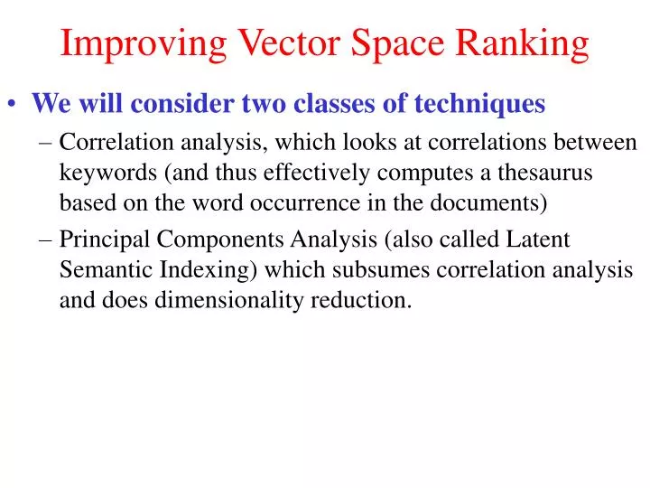
1. Improving Vector Space Ranking • We will consider two classes of techniques • Correlation analysis, which looks at correlations between keywords (and thus effectively computes a thesaurus based on the word occurrence in the documents) • Principal Components Analysis (also called Latent Semantic Indexing) which subsumes correlation analysis and does dimensionality reduction.

2. Correlation/Co-occurrence analysis Co-occurrence analysis: • Terms that are related to terms in the original query may be added to the query. • Two terms are related if they have high co-occurrence in documents. Let n be the number of documents; n1 and n2 be # documents containing terms t1 and t2, m be the # documents having both t1 and t2 If t1 and t2 are independent If t1 and t2 are correlated Measure degree of correlation >> if Inversely correlated

3. Association Clusters • Let Mij be the term-document matrix • For the full corpus (Global) • For the docs in the set of initial results (local) • (also sometimes, stems are used instead of terms) • Correlation matrix C = MMT (term-doc Xdoc-term = term-term) Un-normalized Association Matrix Normalized Association Matrix Nth-Association Cluster for a term tu is the set of terms tv such that Suv are the n largest values among Su1, Su2,….Suk

4. Example 11 4 6 4 34 11 6 11 26 Correlation Matrix d1d2d3d4d5d6d7 K1 2 1 0 2 1 1 0 K2 0 0 1 0 2 2 5 K3 1 0 3 0 4 0 0 Normalized Correlation Matrix 1.0 0.097 0.193 0.097 1.0 0.224 0.193 0.224 1.0 1thAssoc Cluster for K2is K3

5. Scalar clusters Even if terms u and v have low correlations, they may be transitively correlated (e.g. a term w has high correlation with u and v). Consider the normalized association matrix S The “association vector” of term u Au is (Su1,Su2…Suk) To measure neighborhood-induced correlation between terms: Take the cosine-theta between the association vectors of terms u and v Nth-scalar Cluster for a term tu is the set of terms tv such that Suv are the n largest values among Su1, Su2,….Suk

6. Example Normalized Correlation Matrix AK1 USER(43): (neighborhood normatrix) 0: (COSINE-METRIC (1.0 0.09756097 0.19354838) (1.0 0.09756097 0.19354838)) 0: returned 1.0 0: (COSINE-METRIC (1.0 0.09756097 0.19354838) (0.09756097 1.0 0.2244898)) 0: returned 0.22647195 0: (COSINE-METRIC (1.0 0.09756097 0.19354838) (0.19354838 0.2244898 1.0)) 0: returned 0.38323623 0: (COSINE-METRIC (0.09756097 1.0 0.2244898) (1.0 0.09756097 0.19354838)) 0: returned 0.22647195 0: (COSINE-METRIC (0.09756097 1.0 0.2244898) (0.09756097 1.0 0.2244898)) 0: returned 1.0 0: (COSINE-METRIC (0.09756097 1.0 0.2244898) (0.19354838 0.2244898 1.0)) 0: returned 0.43570948 0: (COSINE-METRIC (0.19354838 0.2244898 1.0) (1.0 0.09756097 0.19354838)) 0: returned 0.38323623 0: (COSINE-METRIC (0.19354838 0.2244898 1.0) (0.09756097 1.0 0.2244898)) 0: returned 0.43570948 0: (COSINE-METRIC (0.19354838 0.2244898 1.0) (0.19354838 0.2244898 1.0)) 0: returned 1.0 Scalar (neighborhood) Cluster Matrix 1.0 0.226 0.383 0.226 1.0 0.435 0.383 0.435 1.0 1thScalar Cluster for K2is still K3

7. Similarity Thesaurus • The similarity thesaurus is based on term to term relationships rather than on a matrix of co-occurrence. • obtained by considering that the terms are concepts in a concept space. • each term is indexed by the documents in which it appears. • Terms assume the original role of documents while documents are interpreted as indexing elements

8. Beyond Correlation analysis: PCA/LSI • Suppose I start with documents described in terms of just two key words, u and v, but then • Add a bunch of new keywords (of the form 2u-3v; 4u-v etc), and give the new doc-term matrix to you. Will you be able to tell that the documents are really 2-dimensional (in that there are only two independent keywords)? • Suppose, in the above, I also add a bit of noise to each of the new terms (i.e. 2u-3v+noise; 4u-v+noise etc). Can you now discover that the documents are really 2-D? • Suppose further, I remove the original keywords, u and v, from the doc-term matrix, and give you only the new linearly dependent keywords. Can you now tell that the documents are 2-dimensional? • Notice that in this last case, the true dimensions of the data are not even present in the representation! You have to re-discover the true dimensions as linear combinations of the given dimensions. • The fact that keywords in the documents are not actually independent, and that they have synonymy and polysemy among them, often manifests itself as if some malicious oracle mixed up the data as above. • Need Dimensionality Reduction Techniques • If the keyword dependence is only linear (as above), a general polynomial complexity technique called Principal Components Analysis is able to do this dimensionality reduction • PCA applied to documents is called Latent Semantic Indexing • If the dependence is nonlinear, you need non-linear dimensionality reduction techniques (such as neural networks); much costlier. added

9. Visual Example Classify Fish Length Height

10. Better if one axis accounts for most data variation What should we call the red axis? Size (“factor”)

11. Reduce Dimensions What if we only consider “size” We retain 1.75/2.00 x 100 (87.5%) of the original variation. Thus, by discarding the yellow axis we lose only 12.5% of the original information.

12. 2/5 Project 1 given LSI discussion continued

13. If you can do it for fish, why not to docs? • We have documents as vectors in the space of terms • We want to • “Transform” the axes so that the new axes are • “Orthonormal” (independent axes) • Can be ordered in terms of the amount of variation in the documents they capture • Pick top K dimensions (axes) in this ordering; and use these new K dimensions to do the vector-space similarity ranking • Why? • Can reduce noise • Can eliminate dependent variabales • Can capture synonymy and polysemy • How? • SVD (Singular Value Decomposition)

14. Terms and Docs as vectors in “factor” space In addition to doc-doc similarity, We can compute term-term distance Document vector Term vector • If terms are independent, the • T-T similarity matrix would • be diagonal • =If it is not diagonal, we can • use the correlations to add • related terms to the query • =But can also ask the question • “Are there independent • dimensions which define the • space where terms & docs are • vectors ?”

15. Overview of Latent Semantic Indexing factor-factor (+ve sqrt of eigen values of d-t*d-t’or d-t’*d-t; both same) Doc-factor (eigen vectors of d-t*d-t’) (term-factor)T (eigen vectors of d-t’*d-t) Term Term dt df dfk dtk tft doc ff tfkt ffk Þ doc Reduce Dimensionality: Throw out low-order rows and columns Recreate Matrix: Multiply to produce approximate term- document matrix. dtk is a k-rank matrix That is closest to dt Singular Value Decomposition Convert doc-term matrix into 3matrices D-F, F-F, T-F Where DF*FF*TF’ gives the Original matrix back

16. New document coordinates U*S t1= database t2=SQL t3=index t4=regression t5=likelihood t6=linear F-F D-F 6 singular values (positive sqrt of eigen values of MM’ or M’M) T-F Eigen vectors of MM’ (Principal document directions) Eigen vectors of M’M (Principal term directions)

17. t1= database t2=SQL t3=index t4=regression t5=likelihood t6=linear For the database/regression example Suppose D1 is a new Doc containing “database” 50 times and D2 contains “SQL” 50 times

18. LSI Ranking… • Given a query • Either add query also as a document in the D-T matrix and do the svd OR • Convert query vector (separately) to the LSI space • DFq*FF=q*TF • this is the weighted query document in LSI space • Reduce dimensionality as needed • Do the vector-space similarity in the LSI space

19. Using LSI Can be used on the entire corpus First compute the SVD of the entire corpus Store first k columns of the df*ff matrix [df*ff]k Keep the tf matrix handy When a new query q comes, take the k columns of q*tf Compute the vector similarity between [q*tf]k and all rows of [df*ff]k, rank the documents and return Can be used as a way of clustering the results returned by normal vector space ranking Take some top 50 or 100 of the documents returned by some ranking (e.g. vector ranking) Do LSI on these documents Take the first k columns of the resulting [df*ff] matrix Each row in this matrix is the representation of the original documents in the reduced space. Cluster the documents in this reduced space (We will talk about clustering later) MANJARA did this We will need fast SVD computation algorithms for this. MANJARA folks developed approximate algorithms for SVD Added based on class discussion

20. SVD Computation complexity • For an mxn matrix SVD computation is • O( km2n+k’n3) complexity • k=4 and k’=22 for best algorithms • Approximate algorithms that exploit the sparsity of M are available (and being developed)

21. Bunch of Facts about SVD • Relation between SVD and Eigen value decomposition • Eigen value decomp is defined only for square matrices • Only square symmetric matrices have real-valued eigen values • SVD is defined for all matrices • Given a matrix M, we consider the eigen decomposion of the correlation matrices MMT and MTM. SVD is the eigen vectors of MMT *positive square roots of eigen values of MMT * eigen vectors of MTM • Both MMT and MTM are symmetric (they are correlation matrices) • They both will have the same eigen values • Unless M is symmetric, MMT and MTM are different • So, in general their eigen vectors will be different (although their eigen values are same) • Since SVD is defined in terms of the eigen values and vectors of the “Correlation matrices” of a matrix, the eigen values will always be real valued (even if the matrix M is not symmetric). • In general, the SVD decomposition of a matrix M equals its eigen decomposition only if M is both square and symmetric Added based on the discussion in the class Optional

22. SVD, Rank and Dimensionality Suppose we did SVD on a doc-term matrix d-t, and took the top-k eigen values and reconstructed the matrix d-tk. We know d-tk has rank k (since we zeroed out all the other eigen values when we reconstructed d-tk) There is no k-rank matrix M such that ||d-t –M|| < ||d-t – d-tk|| In other words d-tk is the best rank-k (dimension-k) approximation to d-t! This is the guarantee given by SVD! Rank of a matrix M is defined as the size of the largest square sub-matrix of M which has a non-zero determinant. The rank of a matrix M is also equal to the number of non-zero singular values it has Rank of M is related to the true dimensionality of M. If you add a bunch of rows to M that are linear combinations of the existing rows of M, the rank of the new matrix will still be the same as the rank of M. Distance between two equi-sized matrices M and M’; ||M-M’|| is defined as the sum of the squares of the differences between the corresponding entries (Sum (muv-m’uv)2) Will be equal to zero when M = M’ Optional