Download
1 / 17
200 likes | 419 Views
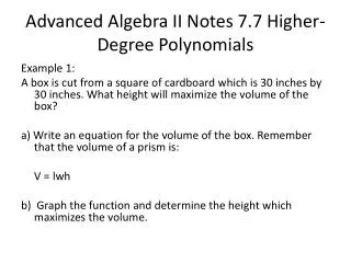
Higher-Degree Polynomials. Lesson 7.7. Polynomials with degree 3 or higher are called higher-degree polynomials.

E N D
Higher-Degree Polynomials Lesson 7.7
Polynomials with degree 3 or higher are called higher-degree polynomials. • If you create a box by removing small squares of side length x from each corner of a square piece of cardboard that is 30 inches on each side, the volume of the box in cubic inches is modeled by the function y=x(30-2x)2, or y=4x3-120x2 +900x. The zero-product property tells you that the zeros are x=0 or x=15, the two values of x for which the volume is 0.
The shape of this graph is typical of the higher-degree polynomial graphs you will work with in this lesson. • Note that this graph has one local maximum at (5, 2000) and one local minimum at (15, 0). • These are the points that are higher or lower than all other points near them.
You can also describe the end behavior—what happens to f (x) as x takes on extreme positive and negative values. In the case of this cubic function, as x increases, y also increases. As x decreases, y also decreases.
Graphs of all polynomials with real coefficients have a y-intercept and possibly one or more x-intercepts. • You can also describe other features of polynomial graphs, such as • local maximums or minimums and end behavior. • Maximums and minimums, collectively, are called extreme values.
The Largest Triangle • Take a sheet of notebook paper and orient it so that the longest edge is closest to you. Fold the upper-left corner so that it touches some point on the bottom edge. Find the area, A, of the triangle formed in the lower-left corner of the paper. • What distance, x, along the bottom edge of the paper produces the triangle with the greatest area?
The Largest Triangle • Work with your group to find a solution. You may want to use strategies you’ve learned in several lessons in this chapter. Write a report that explains your solution and your group’s strategy for finding the largest triangle. Include any diagrams, tables, or graphs that you used. b-y y
Example A • Find a polynomial function whose graph has x-intercepts 3, 5, and -4, and y-intercept 180. Describe the features of its graph. A polynomial function with three x-intercepts has too many x-intercepts to be a quadratic function. It could be a 3rd-, 4th-, 5th-, or higher-degree polynomial function. Consider a 3rd-degree polynomial function, because that is the lowest degree that has three x-intercepts. Use the x-intercepts to write the equation y=a(x-3)(x-5)(x+4), where a≠0.
Substitute the coordinates of the y-intercept, (0, 180), into this function to find the vertical scale factor. • 180=a(0-3)(0-5)(0+4) • 180=a(60) • a=3 • The polynomial function of the lowest degree through the given intercepts is • 180=3(x-3)(x-5)(x+4) • Graph this function to confirm your answer and look for features.
This graph shows a local minimum at about (4, 24) because that is the lowest point in its immediate neighborhood of x-values. • There is also a local maximum at about (1.4, 220) because that is the highest point in its immediate neighborhood of x-values. • Even the small part of the domain shown in the graph suggests the end behavior. As x increases, y also increases. As x decreases, y also decreases. • If you increase the domain of this graph to include more x-values at the right and left extremes of the x-axis, you’ll see that the graph does continue this end behavior.
You can identify the degree of many polynomial functions by looking at the shapes of their graphs. Every 3rd-degree polynomial function has essentially one of the shapes shown below. • Graph A shows the graph of y=x3. It can be translated, stretched, or reflected. • Graph B shows one possible transformation of Graph A. • Graphs C and D show the graphs of general cubic functions in the form y=ax3+bx2+cx+d. • In Graph C, a is positive, and in Graph D, a is negative.
Example B • Write a polynomial function with real coefficients and zeros x=2, x=-5, and x=3+4i. For a polynomial function with real coefficients, complex zeros occur in conjugate pairs, so x=3-4i must also be a zero. In factored form the polynomial function of the lowest degree is y=(x-2)(x+5)[x-(3+4i)][x-(3-4i)] Multiplying the last two factors to eliminate complex numbers gives y=(x-2)(x+5)(x2-6x+25). Multiplying all factors gives the polynomial function in general form: y=x4-3x3-3x2 +135x-250
Graph this function to check your solution. • You can’t see the complex zeros, but you can see x-intercepts 2 and 5.
Any polynomial function of degree n always has n complex zeros (including repeated zeros) and at most n x-intercepts. Remember that complex zeros of polynomial functions with real coefficients always come in conjugate pairs.