Download
1 / 75
750 likes | 919 Views
Network centrality, inference and local computation . Devavrat Shah LIDS+CSAIL+EECS+ORC Massachusetts Institute of Technology. Network centrality. It’s a graph score function Given graph G=(V, E) Assigns “scores” to nodes in the graph That is, F : G R V

E N D
Network centrality, inference and local computation Devavrat Shah LIDS+CSAIL+EECS+ORC Massachusetts Institute of Technology
Network centrality • It’s a graph score function • Given graph G=(V, E) • Assigns “scores” to nodes in the graph • That is, • F: G RV • A given network centrality or graph score function • Designed with aim of solving a certain task at hand
Network centrality: example • Degree centrality • Given graph G=(V, E) • Score of node v is it’s degree • Useful for finding “how connected” each node is • For example, useful for “social clustering” [Parth.-Shah-Zaman’14] 2 4 1 1 3 2
Network centrality: example • Between-ness centrality • Given graph G=(V, E) • Score of node v is proportional to • Number of node pairs whose shortest path pass through it • Represents • “how critical” each node is to keep network connected 0 6.5 4 0 0.5 0
Network centrality: example • PageRank centrality • Given di-graph G=(V, E) • Score of node v is equal to stationary distribution • Of a random walk on the directed graph G • Transition probability matrix of random walk (RW) • If RW at node iat a given time step, it will be at • Node j, with probability Qijwhere • If i has directed edge to j then Qij= (1-α)/di + α/n • Else Qij= α/n
Network centrality: data processing Corpus of Webpages Data (Networked) Decision PageRank Search Relevant Content Scientific Importance H-index Citation Data Why (or why not) does a given centrality make sense?
Statistical data processing • Example task: transmit a MSG bit B (= 0 or 1) • Tx : BBBBB • Rx : Each bit is flipped with probability p (=0.1) • At Rx, using received message, decide whether • Intended MSG is 0 or 1 • ML estimation: • “Majority” Rule Data Statistical Model Decision
Statistical data processing • Data to Decision • Posit model connecting data to decision (variables) • Learn the model • Subsequently make decisions • For example, solve a stochastic optimization problem Data Statistical Model Decision
This talk • Network centrality • Statistical view • For processing networked data • Graph score function = appropriate likelihood function • Explain this view through • Searching source of “information”/”infection” spread • Rumor centrality • Other examples in later talks • Rank centrality • Crowd centrality • Local computation • Stationary probability of a given node in a graph
1854 London Cholera Epidemic Cholera source x Center of mass Dr. John Snow Can we find the source in a network?
Searching for source • Stuxnet (and Duqu) worm: who started it ?
Cyber-attacks Searching for source • Viral epidemics • Social trends
Searching for source Data Statistical Model Decision Infected Nodes, Network How Likely Each Node as Source ?
Model: Susceptible Infected (SI) • Uniform probability of any node being source a priori • Spreading times on each edge are i.i.d random variables. • We will assume an exponential distribution (to develop intuition) • Results will hold for generic distribution (with no atom at 0)
Rumor Source Estimator P(G|source=v) • Not obvious how to calculate it G v We know the rumor graph G We want to find the likelihood function:
Rumor Spreading Order • Rumor spreading order not known • Only spreading constraints are available 2 1 3 4 1 1 2 3 4 3 4 2 1 3 2 4 More spreading orders = more likely to be source
Regular Trees • Regularity of tree + memory-less property of exponential = all spreading orders are equally likely 2 1 4 3 P(G|source=2) = P(2134|source=2) + P(2143|source=2) = 2 * p(d=3,N=4) New problem: counting spreading orders
Counting Spreading Orders • R(v, G)= number of rumor spreading orders from v on G N=Network size T=Subtree size 1 2 4 3
Rumor Centrality (Shah-Zaman, 2010) • The source estimator is a graph score function • It is the “right” score function for source detection • Likelihood function for regular trees • with exponential spreading times • Can be calculated in linear time
Rumor Centrality and Random Walk 5/7 5/7 1/7 1/7 1/7 1/7 • Random walk withtransition probability • Proportional to size of sub-trees • Stationary distribution = • Rumor Centrality 3/7 1/7 3/7 Stationary probability of visiting node Rumor Centrality
Rumor Centrality : General Network Rumor spreads on an underlying spanning tree of graph Breadth-first search tree: “most likely” tree Fast rumor spreading Precisely, “next hop” info required under shortest path routing !
Precision of Rumor Centrality Rumor centrality (normalized) True rumor source 1.0 0.8 0.6 0.4 Estimate of rumor source 0.2 0.0
Precision of Rumor Centrality Rumor centrality (normalized) True rumor source 1.0 0.8 0.6 0.4 Estimate of rumor source 0.2 0.0
Bin Laden Death Twitter Network • Keith Urbahn: first to tweet about the death of Osama bin Laden True rumor source Estimate of rumor source
Effectiveness of rumor centrality • Simulations and examples show • Rumor centrality is useful to find “sources” • Next • When does it work • When it does not work • And, why
Rumor center v*has maximal rumor centrality Source Estimation = Rumor Center Rumor center Tv*j j V* Network is “balanced” around rumor center If rumor spreads in a balanced manner: Source = Rumor Center
Regular Trees (degree=2) • That is, line graphs are hopeless • What about a generic tree ? Balanced sub-trees Proposition [Shah-Zaman, 2010]: Let a rumor spread for a time t on a regular tree with degree d=2 as per the SI model with exponential (or arbitrary) spreading time (with non-trivial variance). Then,
Some Useful Notation • Rumor spreads for time t to n(t) nodes • Let sequence of infected nodes be {v1, v2, …, vn(t)} • v1 = rumor source • Cn(t) = {rumor center is vkafter n(t) nodes are infected} • Cn(t) = correct detection k 1 v1 v2 v4 v3
Number of nodes distance l from any node grows as la(polynomial growth) Result 1: Geometric Trees a=1 Proposition [Shah-Zaman, 2011]: Let a rumor spread for a time t on a (regular) geometric tree with a>0 from a source with degree > 2 as per the SI model with arbitrary spreading times (with exponential moments). Then
Result 2: Regular Trees (degree>2) • Exponential growth • High variance “rumor graph” Theorem [Shah-Zaman, 2011]: Let a rumor spread for a time t on a regular tree with degree d>2 as per the SI model with exponential spreading times. Then where and Ix(a,b) is the regularized incomplete Beta function:
Result 2: Regular Trees (degree>2) 1-ln(2) 3 = 0.25
Result 2: Regular Trees (degree>2) Theorem [Shah-Zaman, 2011]: Let a rumor spread for a time t on a regular tree with degree d>2 as per the SI model with exponential spreading times. Then
Result 2: Regular Trees (degree>2) With “high probability” estimate is “close” to true source
Result 3: Generic Random Trees • Start from root, each node i has hi children (hi are i.i.d.) h1=3 4 1 h4=3 h2=2 h3=4 3 2 • Theorem [Shah-Zaman, 2012]: : Let a rumor spread for a time t on a random tree with E[hi]>1and E[hi2]< from a source with degree > 2as per the SI model with arbitrary spreading times (non-atomic at 0). Then 8
Implication: Sparse random graphs • Random regular graph regular tree • Erdos-Renyi graph random tree • with hi~ Binomial distribution (Poisson in large limit) • Tree results extend
Erdos-Renyi Graphs • Graph has m nodes, each edge exists independently with probability p=c/m Regular tree (degree = 10,000)
Incorrect Detection T2(t) T3(t) V1 T1(t) “Imbalance”
Evaluating T2(t) • “Standard” approach: • Compute E[Tl(t)] • Show concentration of Tl(t) around its mean E[Tl(t)] • Use it to evaluate • P(Ti(t) > Tj(t)) • Issues • Variance in Tl(t) is of same order as mean • Hence, usual concentration is not useful • Even if it were • it would result in 0/1 style answer (which is unlikely) V1 T3(t) T1(t)
Evaluating T2(t) • An alternative: • Understand ratio • Ti(t)/ Tj(t) • Characterize its limiting distribution • That is, Ti(t)/ Tj(t) W • Use W to evaluate • P(Ti(t) > Tj(t)) = P(W>0.5) • Goal: • How to find W ? V1 T3(t) T1(t)
Evaluating • Initially • T1(0)=0 • T2(0) + T3(0)=0 • Z1(0) = 1 • Z2(0)+Z3(0) = 2 Z’(t) =Z2(t) +Z3(t)= Rumor Boundary of T2(t) +T3(t) V1 T2(t)+T3(t) • First infection • T1(.)=1 • T2(.) + T3(.)=0 • Z1(.) = 2 • Z2(0)+Z3(0) = 2 • Second infection • T1(.)=1 • T2(.) + T3(.)=1 • Z1(.) = 2 • Z2(0)+Z3(0) = 3 • In summary • Z1(t)= T1(t)+1 • Z2(t)+Z3(t) = T2(t) + T3(t) +2 • Therefore, for large t • T1(t)/(T2(t) + T3(t)) equals Z1(t)/(Z2(t) + Z3(t)) • Therefore, track ratio of boundaries T1(t) Z1(t)= Rumor Boundary of T1(t)
Evaluating • Boundary evolution • Two types: Z1(t) and Z’(t) • Each new infection increases • Z1(t) or Z’(t) by +1 • Selection of Z1(t) vs Z’(t): • Z1(t) with prob. Z1(t)/(Z1(t) + Z’(t)) • Z’(t) with prob. Z’(t)/(Z1(t) + Z’(t)) • This is exactly Polya’s Urn • With two types of balls Z’(t) =Z2(t) +Z3(t)= Rumor Boundary of T2(t) +T3(t) V1 T2(t)+T3(t) T1(t) Z1(t)= Rumor Boundary of T1(t)
Evaluating • Boundary evolution = Polya’s Urn • M(t) = Z1(t)/(Z1(t) + Z’(t)) • Converges almost surely to a r.v. W • Goal: P(T1 (t) > (T2(t) + T3(t))) = P(W > 0.5) • W has Beta(1,2) distribution Z’(t) =Z2(t) +Z3(t)= Rumor Boundary of T2(t) +T3(t) V1 T2(t)+T3(t) T1(t) Z1(t)= Rumor Boundary of T1(t)
Probability of correct detection • For generic d-regular tree • The corresponding W is Beta(1/(d-2), (d-1)/(d-2)) • Therefore • Where (with d =1/(d-2))
Generic Trees: Branching Process V1 T1(t)= Subtree Z(t)= Rumor boundary (branching process) Lemma (Shah-Zaman ‘12): For large t, Z(t) proportional to T1(t). T1(t) Z(t) Z(0)=1 T2(t)+…+Tk(t) Z’(t) Z’(0)=k-1
Branching Process Convergence • Following result known for branching processes (cf. Athreya-Ney ‘67) • a is the “Malthusian parameter” • depends on distribution of spreading time and node degree • W is a non-degenerate RV with absolutely continuous distribution • For regular tree, exponential spreading times, W has a Beta distribution
Summary, thus far • Rumor source detection • Useful Graph Score Function: Rumor centrality • Exact likelihood function for certain networks • Can be computed quickly (e.g. using linear iterative algorithm) • Effectiveness • Accurately finds source on essentially • any tree or sparse random graph • any spreading time distribution • What else can it be useful for? • Thesis of Zaman – Twitter Search Engine • Bhamidi, Steele and Zaman ‘13
Computing centrality • Computing centrality is equal to finding • Stationary distribution of random walk on network • For a reasonably many settings, including • PageRank • Rumor centrality • Rank centrality • … • Well, that should be easy
Computing stationary distribution • Power iteration method [cf. Golub-Loan ’96] • It primarily requires centralized computation • Iteratively multiply matrix and vector • 100Gb of RAM will limit matrix size to ~100k • But, a social network can be more than a million • And, web is much larger • So, it’s not that easy
Computing stationary distribution • PageRank specific “local” computation solution • A collection of clever, powerful solutions • Jehet.al. 2003, Fogaraset.al. 2005, Avrachenkovet.al. 2007, Bahmaniet.al. 2010, Borgs et al 2012 • Rely on the fact that • From each node, transition to any other node happens • With probability greater or equal to a known fixed positive constant (α/n) • Do not extend for any random walk or countably infinite graphs