Download
1 / 46
460 likes | 611 Views
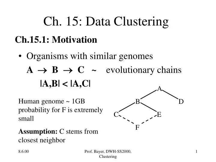
Ch. 15: Data Clustering. Ch.15.1: Motivation. Organisms with similar genomes A B C ~ evolutionary chains |A,B| < |A,C|. A B D C E F. Human genome ~ 1GB probability for F is extremely small Assumption: C stems from closest neighbor. More Examples.

E N D
Ch. 15: Data Clustering Ch.15.1: Motivation • Organisms with similar genomes A B C ~ evolutionary chains |A,B| < |A,C| A B D C E F Human genome ~ 1GB probability for F is extremely small Assumption: C stems from closest neighbor Prof. Bayer, DWH-SS2000, Clustering
More Examples • Stocks with similar behavior in market • Buying basket discovery • Documents on similar topics nearest neighbors? similarity or distance measures? Prof. Bayer, DWH-SS2000, Clustering
Supervised vs. Unsupervised Classification Supervised: set of classes (clusters) is given, assign new pattern (point) to proper cluster, label it with label of its cluster Examples: classify bacteria to select proper antibiotics, assign signature to book and place in proper shelf Unsupervised: for given set of patterns, discover a set of clusters (training set) and assign addtional patterns to proper cluster Examples: buying behavior, stock groups, closed groups of researchers citing each other, more? Prof. Bayer, DWH-SS2000, Clustering
Components of a Clustering Task • Pattern representation (feature extraction), e.g. key words, image features, genes in DNS sequences • Pattern proximity: similarity, distance • Clustering (grouping) algorithm • Data abstraction: representation of a cluster, label for class, prototype, properties of a class • Assessment of quality of output Prof. Bayer, DWH-SS2000, Clustering
Examples • Clustering of documents or research groups by citation index, evolution of papers. Problem: find minimal set of papers describing essential ideas • Clustering of items from excavations according to cultural epoques • Clustering of tooth fragments in anthropology • Carl von Linne: Systema Naturae, 1735, botanics, later zoology • etc ... Prof. Bayer, DWH-SS2000, Clustering
Ch. 15.2: Formal Definitions Pattern: (feature vector, measurements, observations, data points) X = ( x1, ... , xd) d dimensions, measurements, often d not fixed, e.g. for key words Attribute, Feature: xi Dimensionality: d Pattern Set: H = { X1, X2, ... , Xn} H often represented as nd pattern matrix Class: set of similar patterns, pattern generating process in nature, e.g. growth of plants Prof. Bayer, DWH-SS2000, Clustering
More Definitions Hard Clustering: classes are disjoint, every pattern gets a unique label from L = { l1, l2, ... , ln} with li{ 1, ... , k }see Fig. 1 Fuzzy Clustering: pattern Xigets a fractional degree of membership fijfor each output cluster j Distance Measure: metric or proximity function or similarity function in feature space to quantify similarity of patterns Prof. Bayer, DWH-SS2000, Clustering
Ch. 15.3: Pattern Representation and Feature Selection Human creativity: Select few, but most relevant features !!! Cartesian or polar Coordinates? See Fig. 3 Document retrieval: key words (which) or citations? What is a good similarity function? Use of thesaurus? Zoology: Skeleton, lungs instead of body shape or living habits: dolphins, penguins, ostrich!! Prof. Bayer, DWH-SS2000, Clustering
Types of Features • Quantitative: continuous, discrete, intervals, fuzzy • Qualitative: enumeration types (colors), ordinals (military ranks), general features like (hot,cold), (quiet, loud) (humid, dry) • Structure Features: oo hierarchies likevehicle carBenzS400 vehicle boatsubmarine Prof. Bayer, DWH-SS2000, Clustering
Ch. 15.4: Similarity Measures Similar ~ small distance Similarity function: not necessarily a metric, triangle inequality dist (A,B) + dist (B,C) dist (A,C) may be missing, quasi metric. Euclidean Distance dist2 (Xi,Xj) = (k=1d |xi,k - xj,k |²)1/2 = ||Xi - Xj ||2 Special case of Minkowski metric distp (Xi,Xj) = (k=1d |xi,k - xj,k |p)1/p = ||Xi - Xj ||p Prof. Bayer, DWH-SS2000, Clustering
Proximity Matrix: for n patterns with symmetric similarity: n * (n-1)/2 similarity values Representation problem: mixture of continuous and discontinuous attributes, e.g. dist((white, -17), (green, 25)) use wavelength as value for colors and then Euclidean distance??? Prof. Bayer, DWH-SS2000, Clustering
Other Similarity Functions Context Similarity: s(Xi , Xk ) = f(Xi , Xk, E) for environment E e.g. 2 cars on a country road 2 climbers on 2 different towers of 3 Zinnen mountain neighborhood distance of Xkw.r. to Xi = nearest neighbor number = NN(Xi , Xk ) mutual neighborhood distance MND(Xi , Xk ) = NN(Xi , Xk ) + NN(Xk , Xi ) Prof. Bayer, DWH-SS2000, Clustering
Lemma: MND(Xi , Xk ) = MND(Xk , Xi ) MND(Xi , Xi ) = 0 Note: MND is not a metric, triangle inequality is missing! see Fig. 4: NN(A,B) = NN(B,A) = 1 MND(A,B) = 2 NN(B,C) = 2; NN(C,B) = 1 MND(B,C) = 3 see Fig. 5: NN(A,B) = 4; NN(B,A) = 1 MND(A,B) = 5 NN(B,C) = 2; NN(C,B) = 1 MND(B,C) = 3 Prof. Bayer, DWH-SS2000, Clustering
(Semantic) Concept Similarity s (Xi , Xk ) = f (Xi , Xk , C, E) for concept C, environment E Examples for C: ellipse, rectangle, house, car, tree ... See Fig. 6 Prof. Bayer, DWH-SS2000, Clustering
Structural Similarity of Patterns (5 cyl, Diesel, 4000 ccm) (6 cyl, gasoline, 2800 ccm) dist ( ... ) ??? dist (car, boat) ??? how to cluster car engines? Dynamic, user defined clusters via query boxes? Prof. Bayer, DWH-SS2000, Clustering
Ch. 15.5: Clustering Methods • agglomerativemerge clusters versus divisivesplit clusters • monotheticall features at once versus polythetic one feature at a time • hard clusters pattern insingle class versus fuzzy clusterspattern in several classes • incremental add pattern at a time versusnon-increm. add patterns at once (important for large data sets!!) Prof. Bayer, DWH-SS2000, Clustering
Ch. 15.5.1: Hierarchical Clusteringby Agglomeration Single Link: C2 C1 dist (C1, C2) = min { dist (X1, X2 ) : X1C1, X2C2 } Prof. Bayer, DWH-SS2000, Clustering
Complete Link: C2 C1 dist (C1, C2) = max { dist (X1, X2 ) : X1C1, X2C2 } Merge clusters with smallest distance in both cases! Examples: Figures 9 to 13 Prof. Bayer, DWH-SS2000, Clustering
Hierarchical algglomerative clustering algorithmfor single link and complete link clustering 1. Compute proximity matrix between pairs of patterns, initialize each pattern as a cluster 2. Find closest pair of clusters, i.e. sort n2 distances with O(n2*log n), merge clusters, update proximity matrix (how, complexity?) 3. if all patterns are in one cluster then stopelse goto step 2 Note: proximity matrix requires O(n2) space and for distance computation at least O(n2) time for n patterns (even without clustering process), not feasible for large datasets! Prof. Bayer, DWH-SS2000, Clustering
Ch. 15.5.2 Partitioning Algorithms Remember: agglomerative algorithms compute a sequence of partitions from finest (1 pattern per cluster) to coarsest (all patterns in a single cluster). The number of desired clusters is chosen at the end by cutting the dendogram at a certain level. Partitioning algorithms fix the number k of desired clusters first, choose k starting points (e.g. randomly or by sampling) and assign the patterns to the closest cluster. Prof. Bayer, DWH-SS2000, Clustering
Def.: A k-partition has k (disjoint) clusters. There are nk different k-partitions for a set of n patterns. What is a good k-partition? Squared Error Criterion: Assume pattern set H is divided into k clusters labeled by L and li {1, ... ,k} Let cj be the centroid of cluster j, then the squared error is: e2 (H,L) = j=1ki=1nj ||Xij - cj ||2 Xij = jth pattern of cluster j Prof. Bayer, DWH-SS2000, Clustering
Sqared Error Clustering Algorithm (k-means) • 1. Choose k cluster centers somehow • 2. Assign each pattern to ist closest cluster center O(n*k) • 3. Recompute new cluster centers cj’ and e2 • 4. If convergence criterion not satisfied then goto step 2 else exit • Convergence Criteria: • few reassignments • little decrease of e2 Prof. Bayer, DWH-SS2000, Clustering
Problems • convergence, speed of convergence? • local minimum of e2 instead of global minimum? This is just a hill climbing algorithm. • therefore several tries with different sets of starting centroids • Complexities • time: O(n*k*l) l is number of iterations • space: O (n) disk and O(k) main storage space Prof. Bayer, DWH-SS2000, Clustering
Note: simple k-means algorithm is very sensitive to initial choice of clusters -> several runs with different initial choices -> split and merge clusters, e.g. merge 2 clusters with closest centers and split cluster with largest e2 Modified algorithm is ISODATA algorithm: Prof. Bayer, DWH-SS2000, Clustering
ISODATA Algorithm: 1. choose k cluster centers somehow, heuristics 2. assign each pattern to its closest cluster center O(n*k) 3. recompute new cluster centers cj’ and e2 4. if convergence criterion not satisfied then goto step 2 else exit 5. merge and split clusters according to some heuristics Yields more stable results than k-means in practical cases! Prof. Bayer, DWH-SS2000, Clustering
Minimal Spanning Tree clustering 1. Compute minimal spanning tree in O (m*log m) where m is the number of edges in graph, i.e. m = n2 2. Break tree into k clusters by removing the k-1 most expensive edges from tree Ex: see Fig. 15 Prof. Bayer, DWH-SS2000, Clustering
Representation of Clusters hard clusters ~ equivalence classes 1. Take one point as representative 2. Set of members 3. Centroid (Fig. 17) 4. Some boundary points 5. Bounding polygon 6. Convex hull (fuzzy) 7. Decision tree or predicate (Fig. 18) Prof. Bayer, DWH-SS2000, Clustering
Genetic Algorithms with k-means Clustering Pattern setH = { X1, X2, ... , Xn} labeling L = { l1, l2, ... , ln} with li{ 1, ... , k } generate one or several labelings Li to start solution ~ genome or chromosomeB= b1 b2 ... bn B is binary encoding of L with bi = fixed length binary representation of li Note: there are 2 n ld k points in the search space for solutions, gigantic! Interesting cases n >> 100. Removal of symmetries and redundancies does not help much. Prof. Bayer, DWH-SS2000, Clustering
Fitnessfunction: inverse of squared error function. What is the optimum? Genetic operations: crossover of two chromosomes b1 b2 ...| bi ... bn c1 c2 ...|ci ... cn results in two new solutions, decide by fitness function b1 b2 ...| ci ... cn c1 c2 ...| bi ... bn Prof. Bayer, DWH-SS2000, Clustering
Genetic operations continued mutation: invert 1 bit, this guarantees completeness of search procedure. Distance of 2 solutions = number of different bits selection: probabilistic choice from a set of solutions, e.g. seeds that grow into plants and replicate (natural selection). Probabilistic choice of centroids for clustering. exchange of genes replication of genes at another place Integrity constraints for survival (mongolism) and fitness functions for quality. Not all genetic modifications of nature are used in genetic algorithms! Prof. Bayer, DWH-SS2000, Clustering
Example for Crossover S1 = 01000 S2 = 11111 S1 = 01|000 S2 = 11|111 crossover yields S3 = 01111 S4 = 11000 for global search see Fig. 21 Prof. Bayer, DWH-SS2000, Clustering
K-clustering and Voronoi Diagrams C1 C2 C3 C6 C4 C5 Prof. Bayer, DWH-SS2000, Clustering
Difficulties • how to choose k? • how to choose starting centroids? • after clustering, recomputation of centroids • centroids move and Voronoi partitioning changes, e.i. reassignment of patterns to clusters • etc. Prof. Bayer, DWH-SS2000, Clustering
Example 1: Relay stations for mobile phones • Optimal placement of relay stations ~ optimal k-clustering! • Complications: • points correspond to phones • positions are not fixed • number of patterns is not fixed • how to choose k ? • distance function complicated: 3D geographic model with mountains and buildings, shadowing, ... Prof. Bayer, DWH-SS2000, Clustering
Example 2: Placement of Warehouses for Goods • points correspond to customer locations • centroids correspond to locations of warehouses • distance function is delivery time from warehouse multiplied by number of trips, i.e. related to volume of delivered goods • multilevel clustering, e.g. for post office, train companies, airlines (which airports to choose as hubs), etc. Prof. Bayer, DWH-SS2000, Clustering
Ch. 15.6: Clustering of Large Datasets Experiments reported in Literature clustering of 60 patterns into 5 clusters and comparison of various algorithms: using the encoding of genetic algorithms: length of one chromosome: 60 * ceiling(ld(5)) = 180 bits each chromosome ~ 1 solution, i.e. 260*ceiling(ld(5)) = 2180 ~ 100018 ~ 1054 points in the search space for optimal solution Isolated experiments with 200 points to cluster Prof. Bayer, DWH-SS2000, Clustering
Examples clustering pixels of 500500 image = 250.000 points documents in Elektra: > 1 Mio documents see Table 1 above problems prohibitive for most algorithms, only candidate so far is k-means Prof. Bayer, DWH-SS2000, Clustering
Properties of k-means Algorithm • Time O (n*k*l) • Space O (k + n ) to represent H, L, dist (Xi, centroid(li )) • solution is independent of order in which centroids are chosen, order in which points are processed • high potential for parallelism Prof. Bayer, DWH-SS2000, Clustering
Parallel Version 1 use p processors Proci, each Proci knows centroids C1, C2, ...Ck points are partitioned (round robin or hashing) into p groups G1, G2, ... Gp processor Prociprocesses group Gi parallel k-means has time complexity 1/p O(n*k*l) Prof. Bayer, DWH-SS2000, Clustering
Parallel Version 2 Use GA to generate p different initial clusterings C1i, C2i, ... , Cki for i = 1, 2, ... , p Proci computes solution for the seed C1i, C2i, ... , Cki and fitness function for its own solution, which determines the winning clustering Prof. Bayer, DWH-SS2000, Clustering
Large Experiments (main memory) • classification of < 40.000 points, basic ideas: • use random sampling to find good initial centroids for clustering • keep summary information in balanced tree structures Prof. Bayer, DWH-SS2000, Clustering
Algorithms for Large Datasets (on disk) • Divide and conquer: cluster subsets of data separately, then combine clusters • Store points on disk, use compact cluster representations in main memory, read points from disk, assign to cluster, write back with label • Parallel implementations Prof. Bayer, DWH-SS2000, Clustering
Ch. 15.7: Nearest Neighbor Clustering Idea: every point belongs to the same cluster as its nearest neighbor Advantage: instead of computing n2 distances in O(n2 ) compute nearest neighbor in O (n*log(n)) Note: this works in 2-dimensional space with sweep line paradigm and Voronoi diagrams, unknown complexity in multidimensional space Prof. Bayer, DWH-SS2000, Clustering
Nearest Neighbor Clustering Algorithm 1. Initialize: point = its own cluster 2. Compute nearest neighbor Y of X, represent as (X, Y, dist) O(n*log(n)) for 2dimexpected O(n*log(n)) for d dim??? I/O complexity O(n) 3. Sort (X, Y, dist) by dist O (n*log(n)) 4. Assign point to cluster of nearest neighbor ( i.g. merge cluster with nearest cluster and compute: new centroid, diameter, cardinality of cluster, count number of clusters) 5. if not done then goto 2 Prof. Bayer, DWH-SS2000, Clustering
Termination Criteria • distance between clusters • size of clusters • diameter of cluster • squared error function Analysis: with every iteration the number of clusters is decreased to at most 1/2 of previous number, i.e. at most O( log(n)) iterations, total complexity: O(n*log2(n)) resp. O(n*log (n)) we could compute complete dendrogram for nearest neighbor clustering! Prof. Bayer, DWH-SS2000, Clustering
Efficient Computation of Nearest Neighbor 2-dimensional: use sweep line paradigm and Voronoi diagrams d-dimensional: so far just an idea, try as DA? Use generalization of sweep line to sweep zone in combination with UB-tree and caching similar to Tetris algorithm Prof. Bayer, DWH-SS2000, Clustering