Download
1 / 16
170 likes | 332 Views
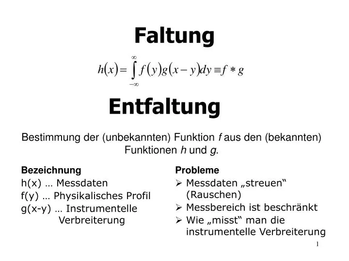
Faltung. Entfaltung. Bestimmung der (unbekannten) Funktion f aus den (bekannten) Funktionen h und g. Bezeichnung h(x) … Messdaten f(y) … Physikalisches Profil g(x-y) … Instrumentelle Verbreiterung. Probleme Messdaten „streuen“ (Rauschen) Messbereich ist beschränkt

E N D
Faltung Entfaltung Bestimmung der (unbekannten) Funktion f aus den (bekannten) Funktionen h und g. Bezeichnung h(x) … Messdaten f(y) … Physikalisches Profil g(x-y) … Instrumentelle Verbreiterung • Probleme • Messdaten „streuen“ (Rauschen) • Messbereich ist beschränkt • Wie „misst“ man die instrumentelle Verbreiterung
Instrumentelle Verzerrung • Spektrale „Reinheit“ der Röntgenstrahlung • Verzerrung an der Beugungsoptik • Nichtkohärente (Compton, Fluoreszenz) und diffuse Streuung Hintergrund Wie bekommt man die instrumentelle Verzerrung? • Berechnung (Näherung) • Messung (Näherung)
Faltungdie Grundmerkmale • Fourier Transformation der Faltung • Faltung einer Funktion mit der Dirac Verteilung
Entfaltungsmethodendie Übersicht • Klassische Stokes Methode mit Gaußschem Glätten der Messdaten • Zerlegen der Messdaten in eine Fourier Reihe • Messdaten werden als eine lineare Kombination der instrumentellen Linienverbreiterung behandelt
Die Stokes Methode Klassisch Modifiziert
Die modifizierte Stokes Methode % Back convolution FF=fft([fy zeros(1,length(gy)-1)]); GG = fft([gy zeros(1,length(fy)-1)]); ht = real(ifft(FF.*GG)); % Fourier transformations HH = fft(hyy); GG = fft(gyy); % Smoothing HH and GG sigma = length(HH)/20; x = 1:length(HH); gauss = exp(-(x.^2)/sigma^2); gauss = gauss + fliplr(gauss); HH = gauss.*HH; sigma = length(GG)/20; % ... the same for GG % Inverse Fourier transform ft = real(ifft(HH./GG)); ft = fftshift(ft);
Die Fourier Reihe Berechnung von Koeffizienten C und S mittels der kleinsten Quadrate
Berechnung von Fourier Koeffizienten Least-square refinement % Harmonic functions fc(jj,:) = cos(jj*omega*hx); fs(jj,:) = sin(jj*omega*hx); % Convolution (g*fc) FF = fft([fc(jj,:) ... zeros(1,length(gyy)-1)]); GG = fft([gyy ... zeros(1,length(fc(jj,:))-1)]); phic(:,jj)=(real(ifft(FF.*GG)))'; % Convolution (g*fs) FF = fft([fs(jj,:) ... zeros(1,length(gyy)-1)]); phis(:,jj)=(real(ifft(FF.*GG)))'; % Calculation of the matrix PHI phic(:,jj) = phic(:,jj)./sigma; phis(:,jj) = phis(:,jj)./sigma; % Solution of the normal equations phi=[ones(length(HH),1)./sigma... phic(:,1:jj) phis(:,1:jj)]; M = phi' * phi; A = (HH./sigma' * phi)'; x = M\B; % Back convolution fy = ... ones(1,length(hy))*P(1)/sum(gy); fy=fy +(P(2:(jj+1)))'*fc(1:jj,:); fy =fy + ... (P((jj+2):(2*jj+1)))'*fs(1:jj,:);
Die lineare Kombination Diskrete Faltung
Die lineare Kombination Voraussetzung: Die Intensitäten weit vom Maximum ist gleich null. Lösung: Die Methode der kleinsten Quadrate % Compose the kernel lh = length(h); for ii = 1:lh , GG(ii,:)=gt((g0-ii+1):(g0-ii+lh)); end % Solve system of linear equations fy = (GG\hy)'*sum(gy);
Vergleich der Entfaltungsmethoden Kritische Fälle: Entfaltung ähnlicher Funktionen und Funktionen mit steilen Flanken
Zusammenfassung • Ein limitierter Faktor ist immer der Grad der Glättung in experimentellen Daten • Lineare Kombination der instrumentellen Profile • Die beste Übereinstimmung zwischen experimentellen und „rekonvoluierten“ Daten / lange Computerzeit • Die Fourier Reihe • Die beste Glättung in den entfalteten Daten / die Methode eignet sich nicht für Profile mit steilen Flanken (sonst zu viele Fourier Koeffizienten notwendig) • Die modifizierte Stokes Methode • Die kürzeste Rechenzeit (sehr schnell mit FFT) / zusätzliche Glättung der Messdaten notwendig (data preprocessing)