Download
1 / 16
160 likes | 170 Views
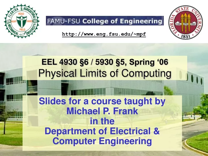
http://www.eng.fsu.edu/~mpf. EEL 4930 §6 / 5930 §5, Spring ‘06 Physical Limits of Computing. Slides for a course taught by Michael P. Frank in the Department of Electrical & Computer Engineering. Course Introduction Moore’s Law vs. Modern Physics Foundations

E N D
http://www.eng.fsu.edu/~mpf EEL 4930 §6 / 5930 §5, Spring ‘06Physical Limits of Computing Slides for a course taught byMichael P. Frankin the Department of Electrical & Computer Engineering
Course Introduction Moore’s Law vs. Modern Physics Foundations Required Background Material in Computing & Physics Fundamentals The Deep Relationships between Physics and Computation IV. Core Principles The two Revolutionary Paradigms of Physical Computation V. Technologies Present and Future Physical Mechanisms for the Practical Realization of Information Processing VI. Conclusion Physical Limits of ComputingCourse Outline Currently I am working on writing up a set of course notes based on this outline,intended to someday evolve into a textbook M. Frank, "Physical Limits of Computing"
Part II. Foundations • This first part of the course quickly reviews some key background knowledge that you will need to be familiar with in order to follow the later material. • You may have seen some of this material before. • Part II is divided into two “chapters:” • Chapter II.A. The Theory of Information and Computation • Chapter II.B. Required Physics Background M. Frank, "Physical Limits of Computing"
Chapter II.A. The Theory of Information and Computation • In this chapter of the course, we review a few important things that you need to know about: • §II.A.1. Combinatorics, Probability, & Statistics • §II.A.2. Information & Communication Theory • §II.A.3. The Theory of Computation M. Frank, "Physical Limits of Computing"
Section II.A.3. The Theory of Computation • In the previous section, we: • Discussed what information is, and how do you quantify it, • Defined entropy as unknown or incompressible information • Now how about the manipulation of information? • I.e., computation, or information processing? • This is the subject of the theory of computing. • A major field of academic research at many universities. • Two major subdivisions of the theory of computing: • (a) The Theory of Computability • What problems can be solved by machine at all? • (b) The Theory of Computational Complexity • How much resources are required to solve a given problem? M. Frank, "Physical Limits of Computing"
Subsection II.A.3.a: Theory of Computability Universal Models of Computation,Uncomputable Functions
Theory of Computability • Emerged out of pioneering work in the 1930s: • Alonzo Church’s Recursive Function Theory • Showed how simple lambda calculus expressions could form a sort of universal programming language. • E.g., factorial function: F = λn.[If (n=0) then 1, else nF(n−1)]. • Emil Post’s String Rewriting Systems • Showed you can use a facility similar to macro-expansion as a universal programming language. • Alan Turing’s Turing Machines. • Model of a simple-minded clerk following explicit instructions and writing/erasing information in squares on graph paper. • All of these systems were shown to be equivalent in their computational power! • They all can compute the very same set of functions. M. Frank, "Physical Limits of Computing"
Church-Turing Thesis • Postulate.Church-Turing Thesis. Any function that can be computed can be computed by an expression of Recursive Function Theory. • Or equivalently, by a Turing machine. • This was originally thought to be a conjecture about mathematics… • But one can easily construct abstract mathematical models of computation that are explicitly defined to violate it… • E.g., let the model “magically” compute uncomputable functions… • But, more profoundly, the Church-Turing thesis is really a statement about physics… • It says, “Any function that can be computed by any physical system in our universe can be computed by a recursive function (equiv. Turing machine)…” • This is true, as far as we know today… M. Frank, "Physical Limits of Computing"
Uncomputable Functions • Certain functions are uncomputable, e.g.: • To solve any given differential equation • To answer of any given mathematical theorem, • Does this theorem have a proof, or not? • First example that was proven uncomputable: • The “Halting Problem” • Does a given program P ever halt? • Or, does it enter an infinite loop? • Or, special case: • Given a Turing machine P, does P eventually halt when given itself as input? • Suppose you had a halt-detector H(P) = “P(P) will halt.” • Consider a derived program B(P), defined as follows: • If H(P)=True, then enter an infinite loop, else halt. • H(B) must give the wrong answer as to whether B(B) will halt, • since B is programmed to simply do the opposite of whatever H would predict it would do! M. Frank, "Physical Limits of Computing"
Subsection II.A.3.b: Theory of Computational Complexity Complexity Metrics, Orders of Growth, Complexity Classes
Computational Complexity Theory • Computability theory asks, • “What functions can be computed at all?” • Given unbounded resources. • This was essentially a solved problem by the 1940s. • Complexity theory asks, • “What amount of computational resources are required to compute a given function?” • In the context of a given model of computation. • This is an active and ongoing area of research. • Some basic topics: • (i) Complexity metrics • (ii) Orders of growth • (iii) Complexity classes M. Frank, "Physical Limits of Computing"
Complexity Metrics • Complexity theory begins with a complexity metric or cost model, • What kind of computational resources are we going to try to quantify, • And how do we quantify them? • Some popular complexity metrics: • “Time” • Number of operations in a serial computation. • Number of parallel steps in a parallel computation. • “Space” • Maximum number of memory cells occupied at any point in the computation. • Less popular today, but often more important in reality: • “Spacetime” • Space used, times parallel steps taken • “Energy” • Number of logic operations times energy consumed per operation. M. Frank, "Physical Limits of Computing"
Order-of-Growth Notation • Usually in complexity theory, we are concerned with which of two models or algorithms has lower complexity in the limit of large problem size • This is usually easier to analyze than trying to decide which is better in a particular case. • Mathematical order-of-growth notation turns out to be convenient for this. • O(f) – An (abstract) function that grows no faster than f. • o(f) – A function that grows strictly more slowly than f. • Ω(f) – A function that grows no slower than f. • ω(f) – A function that grows strictly faster than f. • Θ(f) – A function that grows as fast as f. • That is, it is both O(f) and Ω(f). • Order of growth notation ignores constant factors. • Sometimes this can lead to misleading results M. Frank, "Physical Limits of Computing"
Complexity Example • We often focus on worst-case complexity • Complexity for a worst-case instance of a given size • Although average-case is often important also • E.g., insertion sort has worst-case time complexity T(n) = Θ(n2). • Because it makes n passes through the data, and on average each one looks at Θ(n) items in the worst case. • Quicksort has worst-case time complexity of T(n) = Θ(n log n). • It operates with Θ(log n) levels of recursion • It’s like an indefinite log, in that the base doesn’t matter, • Since it just influences the result by a constant factor • At each level of recursion there’s a total of Θ(n) work • As a result of the different orders of growth, • even a sloppy implementation of quicksort on a slow computer will be faster than a tight implementation of insertion sort on a fast computer… • That is, it will be faster for large enough values of n… M. Frank, "Physical Limits of Computing"
Complexity Classes • A complexity class is the set of all problems that can be solved within a certain order of growth of complexity… • With a certain complexity metric in the context of a certain model of computation… • E.g., the class TIME(n2) is the set of all problems that can be solved with time complexity O(n2) in the input size n. • This set depends on the model of computation used. • We can reduce the model-dependence by ignoring “minor” details such as the precise order of a polynomial O(nk): • P = The union of TIME(nk) for all k • PSPACE = The union of SPACE(nk) for all k. • P is a subset of PSPACE • So-called “nondeterministic” (really super-lucky, most likely unrealistic) models of computation basically ask, • “If the machine randomly guessed the answer to the problem, how many resources would it require simply to verify that its answer was correct?” • It’s a sort of “complexity theory for leprechauns” • NP = The union of NTIME(nk) for all k (time in nondeterministic models) • PNPPSPACE • But, famous unsolved problem: Is P=NP, or is PNP (proper subset)? • No one has managed to prove that our job is any harder than the leprechaun’s! • Maybe there’s some short-cut for finding solutions that no one has discovered yet… PSPACE P M. Frank, "Physical Limits of Computing"
NP-Completeness • Certain problems in the class NP have been proven to be “as hard as any problem in NP” • In the sense that any problem in NP can be easily translated into a problem of this type • So if we could solve problems of this type quickly, then we could solve any problem in NP quickly. • So if any problem of this type is in P, then P=NP. • These problems are called the NP-complete problems. • Examples: • TSP = Traveling Salesman Problem, • SAT = Satisfiability of Boolean Formulas • Other problems in NP aren’t known to be in P, but aren’t known to be NP-complete either… • Example: Factoring of large integers. • But we’ll see later that factoring does have a poly-time quantum algorithm! M. Frank, "Physical Limits of Computing"