Download
1 / 24
240 likes | 442 Views
Linear Sorts. Counting sort Bucket sort Radix sort. Linear Sorts. We will study algorithms that do not depend only on comparing whole keys to be sorted. Counting sort Bucket sort Radix sort. Counting sort. Assumptions: n records Each record contains keys and data

E N D
Linear Sorts Counting sort Bucket sort Radix sort
Linear Sorts • We will study algorithms that do not depend only on comparing whole keys to be sorted. • Counting sort • Bucket sort • Radix sort
Counting sort • Assumptions: • n records • Each record contains keys and data • All keys are in the range of 1 to k • Space • The unsorted list is stored in A, the sorted list will be stored in an additional array B • Uses an additional array C of size k
Counting sort • Main idea:1. For each key value i, i = 1,…,k, count the number of times the keys occurs in the unsorted input array A. Store results in an auxiliary array, C 2. Use these counts to compute the offset. Offseti is used to calculate the location where the record with key value i will be stored in the sorted output list B. The offseti value has the location where the last keyi . • When would you use counting sort? • How much memory is needed?
Counting-Sort( A, B, k)1. fori 1 tok2. doC[i ] 03. forj 1 tolength[A]4. doC[A[ j ] ] C[A[ j ] ] + 15. fori 2 to k6. doC[i ] C[i ] +C[i -1]7. forj length[A] down 18. doB [ C[A[ j ] ] ] A[ j ] 9. C[A[ j ] ] ] C [A[ j ] ] -1 Input: A [ 1 .. n ],A[J] {1,2, . . . , k } Output: B [ 1 .. n ], sorted Uses C [ 1 .. k ],auxiliary storage Counting Sort Analysis: Adapted from Cormen,Leiserson,Rivest
1 2 3 4 5 6 4 1 3 4 3 4 A Counting-Sort( A, B, k)1. fori 1 tok2. doC[i ] 03. forj 1 tolength[A]4. doC[A[ j ] ] C[A[ j ] ] + 15. fori 2 to k6. doC[i ] C[i ] +C[i -1] k = 4, length = 6 C 0 0 0 0 after lines 1-2 C 1 0 2 3 after lines 3-4 C 1 1 3 6 after lines 5-6
1 2 3 4 5 6 4 1 3 4 3 4 A 7. forj length[A] down 18. doB [ C[A[ j ] ] ] A[ j ] 9. C[A[ j ] ] ] C [A[ j ] ] -1 1 2 3 4 5 6 B <- - 3 - -> <-1-> <- - - 4 - -> C 1 1 3 6
B Counting sort A C C C 3 Clinton 4 Smith 1 Xu 2 Adams 3 Dunn 4 Yi 2 Baum 1 Fu 3 Gold 1 Lu 1 Land 1 Lu 1 Land 3 Gold 1 2 3 4 5 6 7 8 9 10 11 1 2 3 4 5 6 7 8 9 10 11 0 0 0 0 4 2 3 2 (4)(3)2 6 (9)8 11 1 2 3 4 1 2 3 4 1 2 3 4 finalcounts "offsets" Original list Sort buckets
Analysis: • O(k + n) time • What if k = O(n) • But Sorting takes (n lg n) ???? • Requires k + n extra storage. • This is a stable sort: It preserves the original order of equal keys. • Clearly no good for sorting 32 bit values.
Bucket sort • Keys are distributed uniformly in interval [0, 1) • The records are distributed into n buckets • The buckets are sorted using one of the well known sorts • Finally the buckets are combined
Bucket sort 1 2 3 4 5 6 7 8 9 10 .78 .17 .39 .26 .72 .94 .21 .12 .23 .68 / / / / / / / / 0 1 2 3 4 5 6 7 8 9 0 1 2 3 4 5 6 7 8 9 .12 .12 .17/ .17/ .21 .23 .23 .21 .26/ .26/ .39/ .39/ .68/ .68/ .78/ .72 .78/ .72 .94/ .94/ Step 2 sorted Step 1 distribute Step3 combine
Analysis • P = 1/n , probability that the key goes to bucket i. • Expected size of bucket is np = n 1/n = 1 • The expected time to sort one bucket is (1). • Overall expected time is (n).
How did IBM get rich originally? • In the early 1900's IBM produced punched card readers for census tabulation. • Cards are 80 columns with 12 places for punches per column. Only 10 places needed for decimals. • Picture of punch card. • Sorters had 12 bins. • Key idea: sort the least significant digit first.
IBM card punching machine Card punching machine
Hollerith’s tabulating machines • As the cards were fed through a "tabulating machine," pins passed through the positions where holes were punched completing an electrical circuit and subsequently registered a value. • The 1880 census in the U.S. took seven years to complete • With Hollerith's "tabulating machines" the 1890 census took the Census Bureau six weeks
Card sorting machine IBM’s card sorting machine
Radixsort • Main idea • Break key into “digit” representation key = id, id-1, …, i2, i1 • "digit" can be a number in any base, a character, etc • Radix sort: for i= 1 to d sort “digit” i using a stable sort • Analysis : (d (stable sort time)) where d is the number of “digit”s
Radix sort • Which stable sort? • Since the range of values of a digit is small the best stable sort to use is Counting Sort. • When counting sort is used the time complexity is (d (n +k )) where k is the range of a "digit". • When k O(n), (d n)
Radix sort- with decimal digits 910 321 572 294 326 178 368 139 139 178 294 321 326 368 572 910 1 2 3 4 5 6 7 8 178 139 326 572 294 321 910 368 910 321 326 139 368 572 178 294 Sorted list Input list
Radix sort with unstable digit sort 13 17 1 2 17 13 17 13 Input list Since unstable and both keys equal to 1 List not sorted
Is Quicksort stable? 48 55 51 48 55 51 1 2 3 51 55 48 KeyData After partition of 0 to 2 After partition of 1 to 2 • Note that data is sorted by key • Since sort unstable cannot be used for radix sort
Is Heapsort stable? 51 55 51 51 55 1 2 Heap Sorted 55 KeyData Complete binary tree, and max heap After swap • Note that data is sorted by key • Since sort unstable cannot be used for radix sort
Example Sort 1 million 64-bit numbers. We could use an in place comparison sort which would run in (n lg n) in the average case. lg 1,000,000 20 passes over the data We can treat a 64 bit number as a 4 digit, radix-216number. So d = 4, k = 216 , n = 1,000,000 (d (n + k )) = ( 4(216 +n)). This takes 4 * 2 passes over the data. 16 bitsd3 16 bitsd2 16 bitsd1 16 bitsdo 64 bits number = d3*(216)3 + d2*(216)2+ d1 (216)1 + d0(216)0 Adapted from Cormen,Leiserson,Rivest