Download
1 / 23
230 likes | 403 Views
Lattice modeling for a storage ring with magnetic field data . X. Huang, J. Safranek (SLAC) Y. Li (BNL) 3/5/2012. Motivation. Discrepancy between original model and measurements. Understanding dynamic effects of rectangular gradient dipoles.

E N D
Lattice modeling for a storage ring with magnetic field data X. Huang, J. Safranek (SLAC) Y. Li (BNL) 3/5/2012 FLS2012, Ring WG, X. Huang
Motivation • Discrepancy between original model and measurements. • Understanding dynamic effects of rectangular gradient dipoles. • Understanding the sources of discrepancies in linear and nonlinear characteristics between models and measurements. • Fringe field of dipoles • Fringe field of quadrupoles • Cross-talk of fields between adjacent magnets? The ideal trajectory in RGD is not a circular arc. Gradient varies with s-variable Off-plane longitudinal field FLS2012, Ring WG, X. Huang
The field-integration approach An AT pass-method that transfer phase space coordinates from one end to the other of a magnetic field region with Bx, By, Bz defined as function of (x, y, z). Equation of motion when using z as free variable. Coordinate transformation at the edges. For dipoles, additional transformation is needed. FLS2012, Ring WG, X. Huang
Magnetic field in a standard SPEAR3 dipole We started examining our lattice model from magnetic fields in magnets. We have coil, wire measurements. Hall probe scans along Z in 2001, 2007. Hall probe scans on X-Z plane in 2007. FLS2012, Ring WG, X. Huang Hall probe x-z scan (2007)
An analytic dipole field model An analytical field model can be built according to general field expansion to obtain the full magnetic field distribution in the dipole. This also removes noise from field measurements. Take the dipole component as an example. Note that the B0/B1 ratio is not constant in the fringe region. FLS2012, Ring WG, X. Huang
Energy calibration How to calibrate the require bending field for a 3GeV beam? + 2001 Z-scan (Yoon, et al, NIMA 2004). The virtual center was held constant (392.35 mm). (Corbett & Tanabe, 2002) This is how dipole magnets were positioned: adjust the dipole current (converted to K-value) until the alignment requirement is met. Following this procedure, the required field integral is calculated to be 1.86420 T-m, with a fixed virtual center, while the measured field integral is 1.86413 T-m for 587.6909 A (operating current since day 1 of SPEAR3). 1.86615 T-m, with the fitted field profile. So the SPEAR3 beam energy may be lower than the nominal value by 0.1%. Energy measurement at SPEAR3 confirmed the prediction with high precision. FLS2012, Ring WG, X. Huang
Effects of quadrupole fringe field A general Hamiltonian (including longitudinal field variation) can be derived using a proper magnetic field expansion(1). J. Irwin, C.X. Wang The leading correction for a hard-edge model is from the last two terms, which are nonlinear(2). The leading correction term from a soft fringe model is linear(3). A perturbation approach * El-Kareh; Forest; Bassetti & Biscari ** Lee-Whiting, Forest & Milutinovic, Irwin & Wang, Zimmermann ***Irwin & Wang (PAC’95), D. Zhou (IPAC10). FLS2012, Ring WG, X. Huang
The linear correction to quadrupole map The correction map J. Irwin, C.X. Wang, PAC95 The generating function for the correction map leading contribution For a symmetric quadrupole, the entrance edge has a reversed sign for I1 matrix The tune changes are (always negative) For SPEAR3, quadrupole fringe fields cause tune changes of [-0.065, -0.059], in agreement with the predictions by the above equation. FLS2012, Ring WG, X. Huang
The nonlinear correction The generating function for the correction map (exit edge) Forest & Milutinovic The function for the entrance edge has an opposite sign. F. Zimmermann derived the average Hamiltonian that include both edges. Hard edge Additional soft edge contribution. 2 is fringe length. and tune dependence on amplitude (only showing hard edge contribution below) This agree with tracking quite well. FLS2012, Ring WG, X. Huang
An AT quadrupole passmethod with fringe field Both linear and nonlinear effects are considered in the new quadrupole passmethod. Forest & Milutinovic pointed out the skew quadrupole part corresponds to a ‘kick map’! A normal quadrupole can thus be modeled by a pair of pi/4 rotation and a kick map. This is the basis for the nonlinear part of the new AT quadrupole pass method. The new quad passmethod agree very well with the field-integration method. FLS2012, Ring WG, X. Huang
The SPEAR3 quadrupole field profile The analytical quadrupole field map for SPEAR3 magnet was based on magnet modeling. Simulated field is converted to an analytic form. Magnetic field All SPEAR3 quads have identical fringe profile. FLS2012, Ring WG, X. Huang
Comparison of models to measurement The model is based on a calibrated experimental lattice with all IDs open (4/6/2009). Effect of the predicted -0.1% beam energy shift is not included, which change the tunes by [0.023, -0.004] for [nux, nuy]. Dipole field is given by the field profile and alignment requirement. Drift lengths neighboring to dipoles adjusted according to measured rf frequency. Strengths of quadrupoles and sextupoles are derived from operating currents and measured excitation curves. No adjustment of any magnet strength! The tune differences are [0.067 -0.060] between the best model and the measurement, a big improvement from the original model. FLS2012, Ring WG, X. Huang
Beta beat and correction Beta beat is relative to the ideal lattice. “No correction” is for “bend field + quad fringe” “corrected” is after the quadrupole strength is adjusted to reduce beta beat (LOCO). Possible causes of optics difference between measurement and un-adjusted model: Interference of magnetic fields between neighboring magnets. Magnet calibration errors. FLS2012, Ring WG, X. Huang
The tune map Chromaticities are corrected with SF/SD to obtain [1.65, 2.18]. Tunes are obtained by tracking 256 turns. “new model” = field model for bend + quad fringe. This model agrees with measurement better. FLS2012, Ring WG, X. Huang
High-order chromaticities * Model chromaticities adjusted to match measured values. ** model chromaticities adjusted, but not yet completely on target. *** improvement from old model. FLS2012, Ring WG, X. Huang
Progress toward fast tracking for dipoles Extract a Lie map from the Taylor map obtained from the field-integration method (Yongjun Li). A map may also be obtained with COSYInfinity. Split the f3 and f4 polynomials into individual terms for tracking (f4 terms are altered by splitting f3), ignore higher order polynomials. Monomial maps have exact solutions (A. Chao, Lie Algrebra Notes). An AT passmethod is written to track f3 (35 terms) and f4 (70 terms) maps (f2 is supplied by a matrix). FLS2012, Ring WG, X. Huang
Comparison of Map-pass to field-pass For comparison, the second order transport map is extracted with AT for the SPEAR3 dipole, using the field-pass or the map-pass. T1ij from the field pass T1ij from the map pass All transverse-only elements agree well (for T2ij, T3ij T4ij, too). The discrepancy for the momentum-related elements may be caused by an problem in the field-pass used for map extraction (different from the one compared to here). The map-pass provides a symplectic tracking solution to the dipole model. FLS2012, Ring WG, X. Huang
Summary and Discussion • We built a lattice model from magnetic field measurements and alignment requirements and compared the linear optics to beam based measurements. • Improved: tunes, betatron functions. • But: still up to 15% maximum beta beat (vertical) • After optics and chromaticity corrections, nonlinear parameters from the model are compared to beam based measurements. • Improved: 2nd order vertical chromaticity, tune map. • But: the tune map is still slightly different from measurement. • We have developed fast symplectic method to represent high order effects. • An accurate model may be crucial for a smooth commissioning of a new machine and for dynamic aperture optimization of existing machines. • Quadrupole fringe field effect (tune shifts and beta beat) would be larger for a large ring (with more quads). • Magnetic field based lattice can be used as a “reference” model. • More efforts are need to understand the discrepancies between model and measurements. FLS2012, Ring WG, X. Huang
This slide is left blank FLS2012, Ring WG, X. Huang
The dipole field map B0, B1, B2 from X-Z scan By(at y=0,z=0) = -1.233257 + 3.143436*x -0.324508*x^2 ByL = -1.857103 + 4.662405*x -0.931245*x^2 Coil measurement gives ByL (T m)= -1.8506 +4.6081 x - 1.2632 x^2 Note that the dipole/quadrupole ratio is constant (392.35 mm) in the magnet body, but varying in the fringe. The integrated quadrupole component is actually 2% weaker than the present model. (The coil measurement gives an average ratio of 399.8+-1.7 mm) FLS2012, Ring WG, X. Huang
The linear correction to quadrupole map A perturbation approach Hard-edge model, for exit edge Perturbation term The map J. Irwin, C.X. Wang, PAC95 The generating function for the correction map (only leading contribution is shown) For a symmetric quadrupole, the entrance edge has a reversed sign for I1 matrix The tune change would be (always negative) FLS2012, Ring WG, X. Huang
Verification of the quad fringe pass method yi=0.005 m Quadpass: quad transfer matrix Quadpass+matrix: quad transfer matrix + linear edge transfer matrix. New quad pass: with linear and nonlinear corrrection. Field pass: integration through magnetic field. With the (quad+matrix) part subtracted. Zimmerman result is from the average Hamiltonian H1+2 FLS2012, Ring WG, X. Huang
A pass method for magnetic field in AT • Coordinate transformation at the entrance and exit of the magnets • Integration of the Lorentz equation in the body of magnets. Can we study beam dynamics with such a pass method? With an accurate magnetic field model, we can reproduce reality in simulation. Integration is slow and non-symplectic, not good for dynamic aperture tracking. But it should be good for linear and nonlinear parameter evaluation.