Implementation of Relational Operations

1. Implementation of Relational Operations R&G - Chapters 12 and 14

2. Introduction • Next topic: QUERY PROCESSING • Some database operations are EXPENSIVE • Huge performance gainst by being “smart” • We’ll see 1,000,000x over naïve approach • Main weapons are: • clever implementation techniques for operators • exploiting relational algebra “equivalences” • using statistics and cost models to choose

3. Simple SQL Refresher • SELECT <list-of-fields> FROM <list-of-tables> WHERE <condition> SELECT S.name, E.cid FROM Students S, Enrolled E WHERE S.sid=E.sid AND E.grade='A'

4. A Really Bad Query Optimizer • For each Select-From-Where query block • Create a plan that: • Forms the cross product of the FROM clause • Applies the WHERE clause • (Then, as needed: • Apply the GROUP BY clause • Apply the HAVING clause • Apply any projections and output expressions • Apply duplicate elimination and/or ORDER BY) spredicates  … tables

5. Cost-based Query Sub-System Catalog Manager Select * From Blah B Where B.blah = blah Queries Query Parser Query Optimizer Plan Generator Plan Cost Estimator Schema Statistics Query Plan Evaluator

6. The Query Optimization Game • Goal is to pick a “good” plan • Good = low expected cost, under cost model • Degrees of freedom: • access methods • physical operators • operator orders • Roadmap for this topic: • First: implementing individual operators • Then: optimizing multiple operators

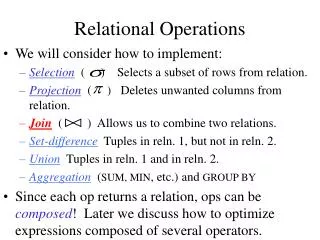
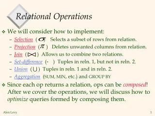
7. Relational Operations • We will consider how to implement: • Selection (  ) Select a subset of rows. • Projection (  ) Remove unwanted columns. • Join ( ) Combine two relations. • Set-difference ( − ) Tuples in reln. 1, but not in reln. 2. • Union (  ) Tuples in reln. 1 and in reln. 2. • Q: What about Intersection?

8. Schema for Examples • Sailors: • Each tuple is 50 bytes long, 80 tuples per page, 500 pages. • [S]=500, pS=80. • Reserves: • Each tuple is 40 bytes, 100 tuples per page, 1000 pages. • [R]=1000, pR=100. Sailors (sid: integer, sname: string, rating: integer, age: real) Reserves (sid: integer, bid: integer, day: dates, rname: string)

9. Simple Selections SELECT * FROM Reserves R WHERE R.rname < ‘C%’ • How best to perform? Depends on: • what indexes are available • expected size of result • Size of result approximated as (size of R) * selectivity • selectivity estimated via statistics – we will discuss shortly.

10. Our options … • If no appropriate index exists: Must scan the whole relation cost = [R]. For “reserves” = 1000 I/Os.

11. Our options … • With index on selection attribute: 1. Use index to find qualifying data entries 2. Retrieve corresponding data records Total cost = cost of step 1 + cost of step 2 • For “reserves”, if selectivity = 10% (100 pages, 10000 tuples): • If clustered index, cost is a little over 100 I/Os; • If unclustered, could be up to 10000 I/Os! … unless … UNCLUSTERED Index entries CLUSTERED direct search for data entries Data entries Data entries (Index File) (Data file) Data Records Data Records

12. Refinement for unclustered indexes 1. Find qualifying data entries. 2. Sort the rid’s of the data records to be retrieved. 3. Fetch rids in order. Each data page is looked at just once (though # of such pages likely to be higher than with clustering). UNCLUSTERED Data entries (Index File) (Data file) Data Records

13. General Selection Conditions • (day<8/9/94 AND rname=‘Paul’) OR bid=5 OR sid=3 • First, convert to conjunctive normal form (CNF): • (day<8/9/94 OR bid=5 OR sid=3 ) AND (rname=‘Paul’ OR bid=5 OR sid=3) • We only discuss the case with no ORs • Terminology: • A B-tree index matches terms that involve only attributes in a prefix of the search key. e.g.: • Index on <a, b, c> matches a=5 AND b= 3, but notb=3.

14. 2 Approaches to General Selections Approach I: • Find the cheapest access path • retrieve tuples using it • Apply any remaining terms that don’t match the index • Cheapest access path: An index or file scan that we estimate will require the fewest page I/Os.

15. Cheapest Access Path - Example query: day < 8/9/94 AND bid=5 AND sid=3 some options: B+tree index on day; check bid=5 and sid=3 afterward. hash index on <bid, sid>; check day<8/9/94 afterward. • How about a B+tree on <rname,day>? • How about a B+tree on <day, rname>? • How about a Hash index on <day, rname>?

16. 2 Approaches to General Selections Approach II: use 2 or more matching indexes. 1. From each index, get set of rids 2. Compute intersection of rid sets 3. Retrieve records for rids in intersection 4. Apply any remaining terms EXAMPLE:day<8/9/94 AND bid=5 AND sid=3 Suppose we have an index on day, and another index on sid. • Get rids of records satisfying day<8/9/94. • Also get rids of records satisfying sid=3. • Find intersection, then retrieve records, then check bid=5.

17. Projection SELECT DISTINCT R.sid, R.bid FROM Reserves R • Issue is removing duplicates. • Use sorting!! 1. Scan R, extract only the needed attributes 2. Sort the resulting set 3. Remove adjacent duplicates Cost: Ramakrishnan/Gehrke writes to temp table at each step! Reserves with size ratio 0.25 = 250 pages. With 20 buffer pages can sort in 2 passes, so: 1000 +250 + 2 * 2 * 250 + 250 = 2500 I/Os

18. Projection -- improved • Avoid the temp files, work on the fly: • Modify Pass 0 of sort to eliminate unwanted fields. • Modify Passes 1+ to eliminate duplicates. Cost: Reserves with size ratio 0.25 = 250 pages. With 20 buffer pages can sort in 2 passes, so: • Read 1000 pages • Write 250 (in runs of 40 pages each) = 7 runs • Read and merge runs (20 buffers, so 1 merge pass!) Total cost = 1000 + 250 +250 = 1500.

19. Other Projection Tricks If an index search key contains all wanted attrs: • Do index-only scan • Apply projection techniques to data entries (much smaller!) If a B+Tree index search key prefix has all wanted attrs: • Do in-order index-only scan • Compare adjacent tuples on the fly (no sorting required!)

20. Joins SELECT * FROM Reserves R1, Sailors S1 WHERE R1.sid=S1.sid • Joins are very common. • R ´ S is large; so, R ´ S followed by a selection is inefficient. • Many approaches to reduce join cost. • Join techniques we will cover today: • Nested-loops join • Index-nested loops join • Sort-merge join

21. Simple Nested Loops Join foreach tuple r in R do foreach tuple s in S do if ri == sj then add <r, s> to result R S: Cost = (pR*[R])*[S] + [R] = 100*1000*500 + 1000 IOs • At 10ms/IO, Total time: ??? • What if smaller relation (S) was “outer”? • What assumptions are being made here? • What is cost if one relation can fit entirely in memory?

22. Page-Oriented Nested Loops Join foreach page bR in R do foreach page bS in S do foreach tuple r in bR do foreach tuple s in bSdo if ri == sj then add <r, s> to result R S: Cost = [R]*[S] + [R] = 1000*500+ 1000 • If smaller relation (S) is outer, cost = 500*1000 + 500 • Much better than naïve per-tuple approach!

23. Block Nested Loops Join . . . • Page-oriented NL doesn’t exploit extra buffers :( • Idea to use memory efficiently: Join Result R & S block of R tuples (B-2 pages) . . . . . . Output buffer Input buffer for S • Cost: Scan outer + (#outer blocks * scan inner) • #outer blocks =

24. Examples of Block Nested Loops Join • Say we have B = 100+2 memory buffers • Join cost = [outer] + (#outer blocks * [inner]) #outer blocks = [outer] / 100 • With R as outer ([R] = 1000): • Scanning R costs 1000 IO’s (done in 10 blocks) • Per block of R, we scan S; costs 10*500 I/Os • Total = 1000 + 10*500. • With S as outer ([S] = 500): • Scanning S costs 500 IO’s (done in 5 blocks) • Per block of S, we can R; costs 5*1000 IO’s • Total = 500 + 5*1000.

25. Index Nested Loops Join lookup(ri) ri R: INDEX on S Data entries sj S: Data Records R S: foreach tuple r in R do foreach tuple s in S where ri == sjdo add <r, s> to result

26. Index Nested Loops Join R S: foreach tuple r in R do foreach tuple s in S where ri == sjdo add <r, s> to result Cost = [R] + ([R]*pR) * cost to find matching S tuples • If index uses Alt. 1, cost = cost to traverse tree from root to leaf. • For Alt. 2 or 3: • Cost to lookup RID(s); typically 2-4 IO’s for B+Tree. • Cost to retrieve records from RID(s); depends on clustering. • Clustered index: 1 I/O perpage of matching S tuples. • Unclustered: up to 1 I/O per matching S tuple.

27. Reminder: Schema for Examples • Sailors: • Each tuple is 50 bytes long, 80 tuples per page, 500 pages. • [S]=500, pS=80. • Reserves: • Each tuple is 40 bytes, 100 tuples per page, 1000 pages. • [R]=1000, pR=100. Sailors (sid: integer, sname: string, rating: integer, age: real) Reserves (sid: integer, bid: integer, day: dates, rname: string)

28. Sort-Merge Join • Sort R on join attr(s) • Sort S on join attr(s) • Scan sorted-R and sorted-S in tandem, to find matches Example: SELECT * FROM Reserves R1, Sailors S1 WHERE R1.sid=S1.sid

29. Cost of Sort-Merge Join Block-Nested-Loop cost = 2500 … 15,000 • Cost: Sort R + Sort S + ([R]+[S]) • But in worst case, last term could be [R]*[S] (very unlikely!) • Q: what is worst case? Suppose B = 35 buffer pages: • Both R and S can be sorted in 2 passes • Total join cost = 4*1000 + 4*500 + (1000 + 500) = 7500 Suppose B = 300 buffer pages: • Again, both R and S sorted in 2 passes • Total join cost = 7500

30. Other Considerations … > < 1. An important refinement: Do the join during the final merging pass of sort ! • If have enough memory, can do: 1. Read R and write out sorted runs 2. Read S and write out sorted runs 3. Merge R-runs and S-runs, and find R S matches Cost = 3*[R] + 3*[S] Q: how much memory is “enough”(will answer next time …) • 2. Sort-merge join an especially good choice if: • one or both inputs are already sorted on join attribute(s) • output is required to be sorted on join attributes(s) • Q: how to take these savings into account?(stay tuned …)

31. Summary • A virtue of relational DBMSs: queries are composed of a few basic operators • The implementation of these operators can be carefully tuned • Many alternative implementation techniques for each operator • No universally superior technique for most operators. • Must consider available alternatives • Called “Query optimization” -- we will study this topic soon!