Download

1 / 75
770 likes | 956 Views
Practical SAT. A Tutorial on Applied Satisfiability Solving. Niklas Eén Cadence Research Laboratories. Presented by Alan Mishchenko UC Berkeley. Overview. Modern SAT solvers – Terminology – Chaff-like SAT solvers – Features of MiniSat Encoding problems to be solved by SAT

E N D
Practical SAT A Tutorial on Applied Satisfiability Solving Niklas Eén Cadence Research Laboratories Presented by Alan Mishchenko UC Berkeley
Overview • Modern SAT solvers • – Terminology – Chaff-like SAT solvers – Features of MiniSat • Encoding problems to be solved by SAT • – Minimum-area AIG synthesis – AIG-to-CNF conversion – CNF minimization • – Incremental SAT interface • Conclusions
Introduction SAT Terminology
Quick Recap SAT problem: Given a CNF, find an assignment of variables that makes at least one literal true in each clause. • In SAT, clauses are written as sets: {a, -b} {b,-c,d} {-d} • A clause CsubsumesC' if C C'. Example: clause {x, y} subsumes clause {x, y, z} Clause (disjunction) Literal Unit Clause (a ∨ ¬b) ∧ (b ∨ ¬c ∨ d) ∧ (¬d) ∧ ... CNF (conjunction of clauses)
Quick Recap (cont.) Boolean Constraint Propagation (BCP): Performing unit resolution until saturation (resolution impossible). • Clauses subsumed by unit clauses are called satisfied, and are removed. • During BCP, unit clauses are stored on the side (not in the clause database). {a, -b} {b, -c, d} resolve(b){a, -c, d}
Quick Recap (cont.) BCP-implication: Variable y is implied by x if adding {x} and performing BCP will derive {y}. Example: adding {a} to{-a, b}, {-a, c}, {-b, -c, d}gives: {b}, {c}, {d}Note, we have a BCP d but not-d BCP -a
dpll(clauses) clauses = bcp(clauses) ifclauses = : return TRUE // Problem is SAT ifclauses: return FALSE // Conflict pick x from Vars(clauses) returndpll(clauses {-x}) dpll(clauses {x}) DPLL • The unit clauses found during BCP form a partial assignment
Modern SAT Solvers Chaff-like SAT solvers
Chaff-like SAT Solvers • Not DPLL: • No variable flipping, no search tree • Trying to build a resolution proof of UNSAT • Conflicts are guiding the proof • Two heuristics help each other: • Activity based variable heuristic • Variable state independent decaying sum (VSIDS) • Conflict clause generation • Together with 2-watched literal scheme, these two heuristics make a “Chaff-like SAT solver”.
Chaff-like SAT Solvers forever{ // no termination conditions bcpif no conflict { make decision} else { analyze conflict undo assignments add conflict clause}}
Chaff-like SAT Solvers forever{ bcpif no conflict { if no unassigned variable { return SAT } make decision} else { if no decisions made { return UNSAT } analyze conflict undo assignments add conflict clause}}
Chaff-like SAT Solvers forever{ bcpif no conflict { if no unassigned variable { return SAT } if enough conflicts { restart } if top-level { simplify clause database } if too many conflict clauses { remove inactive } make decision} else { if no decisions made { return UNSAT }analyze conflict undo assignments add conflict clause}}
Conflict Clauses − Intuition Pigeon Hole: _ _ _ _ x1x2 x1x2 x1x2 x1x2 1: 1 2 3 2: -1 -2 3: -1 -3 4: -2 -3 5: 1 2 4 6: -1 -2 7: -1 -4 8: -2 -4 9: 1 3 4 10: -1 -3 11: -1 -4 12: -3 -4 13: 2 3 4 14: -2 -3 15: -2 -4 16: -3 -4 _ _ x3x4 _ x3x4 x3x4 _ x3x4 17: -2 3 4 (2 9) 18: 3 4 (13 17) ... 22: 3 23:
Conflict Clauses and BCP • Conflict clauses strengthen BCP until UNSAT can be proven without decisions. Example: Adding conflict clause¬a ¬b ¬cprovides three new BCP implications:a b BCP ¬c a c BCP ¬b b c BCP ¬a By construction, a conflict clause adds at least one new BCP-implication set of consistent partial assigments, closed under BCP, shrinks. completeness of algorithm
_ _ _ a b c d e f g clause42: watch 0 watch 1 State Variables clauses : {Clause}Set of clauses of size ≥ 2 assign : Var BoolDuring search, current partial assignment to variables.Initially stores all unit clauses (“top-level” assignments) watch : Lit {Clause}Clauses to visit when a literal becomes FALSE. clause42 ∈watch(a) _ clause42 ∈watch(b)
. . . State Variables (cont.) trail : <Lit>Sequence of literals forming an assignment stack.Different decision levels are separated: reason : Var ClauseFor each assigned variable, the clause it propagated from.Unassigned / decision / top-level variables map to . level : Var IntThe decision level when the variable became assigned. _ _ _ level 0:x9 x4 x5 x6 x7level 1:x8 x0 x3 _
State Variables (cont.) activity : Var FloatShows how active the variable was in conflict clause derivation. heap : <Var>Priority queue with most active variable on top.
Main Purpose of Variables LEARNING:reasonlevel DECISION:activityheap PROPAGATION:clausesassignwatch UNDO:trail
. . . _ _ _ _ _ _ a b c d e f g c b a d e f g Propagation • Trail is used as a propagation queue • 2-literal watching scheme (red literals false):If cannot find a new watch, clause is either unit (propagate) or conflicting (analyze) _ _ _ level 8:x1 x8 x4 x6 x23 x42 Head of Prop. Queue
Conflict Analysis • “Algorithm”: • Start with the ⊥-node as the frontier. • Repeatedly replace one node of the frontier with all its predecessors. • “Algorithm” Algorithm: • Which node to replace • When to stop
Conflict Analysis • Which node to replace? • A topological order will avoid reintroducing eliminated nodes. • The trail is a topological order.
Conflict Analysis • When to stop? • If we use conflict clauses to drive backtracking: • Produce a clause that would have propagated at an earlier decision level • Equivalent: Produce a clause with only one literal from the latest decision level. • Two natural points: • Decision variables (maximal) • First UIP (minimal)
Last Decision Level Prev. Decision Levels Conflict Analysis: Example trail:-a;-b c; -d e -f reason(f): { -f -e d b }reason(-e):{ e d -c b a } conf. clause:{ f -e -c } { f -e -c } {-f -e d b }= {-e d -c b } {-e d -c b } { e d -c b a }= { d -c b a }
Things Worth Noting • Conflict nests. • Long clauses are not useless. • Since we are not flipping variables, we can “branch” on the same variable/value twice. • Watches are not moved during backtracking. • Watches tend to migrate to the “silent” literals. • Industrial SAT problem ≈ UNSAT problems
Things Worth Noting (cont.) • Very common to visit satisfied clauses • Restarts are not “real” restarts. Their main function is to compress the trail. Example:a is active, b inactive, clauses: {a,x} {b,x}. • CNF-based is solver "better" than circuit-based: • Clauses, if long, are efficient for BCP • Simple and uniform, which means: • easy to improve algorithm • easy to get correct • beautiful
Modern SAT Solvers Features of MiniSat
Features of MiniSat • Floating point based VSIDS heuristic: • Moves it closer to BerkMin/Siege • Longer memory (“never” decays to zero)1 • Aggressive decay • Variable-based, not literal-based • Bumps a lot of variables in conflict analysis • Polarity heuristic: always try FALSE first 1 With current decay, floating point number becomes epsilon after 14468 conflicts
Features of MiniSat (cont.) • Conflict clause minimization • Based on self-subsuming resolution:{x, A} ⊗x {x, A, B} = {A, B} • Simplest version has trivial implementation:minimizeCC(Clause C) for each p ∈ C doif (reason(p)\{p} ⊆ C) mark p remove all marked literals in C • Can do better (unpublished work of Sörensson)
Features of MiniSat (cont.) • Binary clauses inlined in watcher lists • Progressive restarts (improved by PicoSAT) • Activity based clause deletion • Handles subsumed clauses better than the original scheme • Very effective for small, hard SAT problems • Random decisions are made 2% of the time
Features of MiniSat 2.0 • Improved SATELITE-style preprocessing • Faster, better, more features • Integrated • Indeed, what SATELITE was meant to be...
Conflict Clause Minimization • Continuation of analysis to previous decision levels — but restricted • Finds a minimal subset of the originally derived conflict clause • Typically removes about 30% of the literals of the conflict clause
Conflict Clause Minimization // pre-condition: reason(p) ≠ removable(Lit p, Clause C, Ints L) { S := {p}while S ≠ { pick q ∈S occuring last in trail Z := reason(q) \ {-q} \ Cifr Z such that level(r) ∉ L return FALSE S := S\{q} ∪ Z}return TRUE}L = levels in C = { level(c) | c C } • Optimization 1:Pick q from S occurring last in trail. • Optimization 2:Stop if new level introduced.
SAT Encoding Example: Optimal circuit synthesis
And-Inverter Graphs • Circuits with 2-input AND-gates and inverters • Implementation: Inverters are “free” – just a bit on the edge pointer. Consider the following problem: • For 4-input, 1-output function, find AIG with the minimum number of AND-nodes? Let's try to solve it with SAT...
And-Inverter Graphs Primary Output ? ? ? ? PI3 PI2 PI1 PI0 F 0 0 0 0 0 0 0 0 1 0 0 0 1 0 0 0 0 1 1 0 ⋮ ⋮ 1 1 1 0 0 1 1 1 1 1 Primary Inputs • Let F be the 16-bit truth-table for the desired function to synthesize. • Let N be the number of nodes to use. 1000000000000000 1000100010001000 1111000000000000 1010101010101010 1111000011110000 1100110011001100 1111111100000000
Problem Variables ChildL/R(n,m): • Node m is the left/right child of node n. SignL/R(n): • Node n's left/right child edge has an inverter. InL/R(n,b) • bth bit of input value to node n (after inverter). Out(n,b): • bth bit of output value Out(n,b) Node n InL(n,b) InR(n,b) SignL(n) SignR(n) ChildL(n,m) ChildR(n,m) n,m = Node# ∈[-4,N) (-1..-4 used for primary inputs) b = Bit# ∈ [0,16) (16 possible input combinations) n,m = Node# ∈[-4,N) (-1..-4 used for primary inputs)
Out(n,b) Node n InL(n,b) InR(n,b) SignL(n) SignR(n) ChildL(n,m) ChildR(n,m) n,m = Node#∈[-4,N) b = Bit# ∈ [0,16) Problem Constraints Constraining PIs:n [0, 4) :b [0, 16) :bitSet(n, b) ? Out(-n–1, b) : -Out(-n–1, b) Constraining PO:b[0, 16) :bitSet(F, b) ? Out(N-1, b) : -Out(N-1, b) 1010101010101010 1100110011001100 1111000011110000 1111111100000000 Top Node bitSet(k,m) is true if kth bit of m is 1.
Out(n,b) Node n InL(n,b) InR(n,b) SignL(n) SignR(n) ChildL(n,m) ChildR(n,m) n,m = Node#∈[-4,N) b = Bit# ∈ [0,16) Problem Constraints (cont.) Constraining ANDs:n [0, N) :b[0, 16) :-InL(n,b) -Out(n,b) -InR(n,b) -Out(n,b) InL(n,b) InR(n,b) Out(n,b) How about inputs InL and InR?
(cont.) Out(n,b) Node n InL(n,b) InR(n,b) SignL(n) SignR(n) ChildL(n,m) ChildR(n,m) n,m = Node#∈[-4,N) b = Bit# ∈ [0,16) Problem Constraints • Constraining ANDs:n [0, N) :b [0, 16) :m [-4, n) : • ChildL(n,m) -SignL(n) Out(m,b) InL(n,b)ChildL(n,m) -SignL(n) - Out(m,b) - InL(n,b)ChildL(n,m) SignL(n) Out(m,b) - InL(n,b)ChildL(n,m) SignL(n) - Out(m,b) InL(n,b) • Ditto for: ChildR, SignR, InR
Out(n,b) Node n InL(n,b) InR(n,b) SignL(n) SignR(n) ChildL(n,m) ChildR(n,m) n,m = Node#∈[-4,N) b = Bit# ∈ [0,16) Problem Constraints (cont.) Inputs are one-hot:n [0, N) :oneHot(Ln)oneHot(Rn)whereLn = { ChildL(n,m) | m [-4, n) } Rn = { ChildR(n,m) | m [-4, n) } avoid cycles
Problem Constraints (cont.) oneHot(S):Add S = {s1, s2, ... sk-1} as a clause:s1 s2 ... sk-1Then at most one literal true:i [1, k) :j [0, i) :-si -sj
Out(n,b) Node n InL(n,b) InR(n,b) SignL(n) SignR(n) ChildL(n,m) ChildR(n,m) n,m = Node#∈[-4,N) b = Bit# ∈ [0,16) Problem Constraints (cont.) Right child < Left child:n [0, N) :m [-4, n) :k [m, n) :ChildL(n,m) -ChildR(n,k)
Out(n,b) Node n InL(n,b) InR(n,b) SignL(n) SignR(n) ChildL(n,m) ChildR(n,m) n,m = Node#∈[-4,N) b = Bit# ∈ [0,16) Problem Constraints (cont.) Use all nodes:- All nodes (except the top node)should have at least one parent. Order left children:- For n > m, “left child of n” > “left child of m”. Adjacent pairs constraint: - Two adjacent nodes should have three distinct children.
Problem Constraints (cont.) Even more constraints • Order right children (if left are equal) • Unique truth-tables • Non-trivial truth-tables (cheaper) • Constraints on input permutation/negation (requires different constr on PO)
The Most Complex Functions There are 4 functions that require 10 nodes:
Comments on SAT Formulations • SAT is not magic • Need to consider: • Are there fast specialized algorithms? • How often do we need to solve this problem? • Shape of search space (is it localizable?) • Do variables have symmetries? • Are there constraints with no compact CNF encoding?
Rules of Thumb • Redundant constraints may be important. • Many encodings possible. • Effectiveness may vary greatly. • Avoid bit-vectors. • Avoid XORs. • Small is not always better. Need "good" literals. • Example: Sorters vs. adders in PB-translation
SAT Encoding Converting circuits to CNF
1 2 3 4 5 6 Tseitin Transformation t = AND(x, y) • {x, ¬t} {y, ¬t} {¬x, ¬y, t} t = MUX(s, x, y) • {¬s, ¬x, t} {¬s, x, ¬t} {s, ¬y, t} {s, y, ¬t} • {¬x, ¬y, t} {x, y, ¬t} Clauses 5 and 6 logically redundant: • 1 s 3 = 5 • 2 s 4 = 6 but add strength to BCP.
AIG CNF • Big conjunctions: a (b (c d)) • Only introduce a variable for the top-node(unless AND-node is shared). • In this case: 9 clauses 5 clauses • MUXs: MUX(s,x,y) = (s x) (-s y) • 9 clauses instead of 4 (or 6 with redundants). • XORs: • XOR(x,y) = MUX(x, y, -y) • always 4 clauses (redundant clauses trivial)