Download

1 / 50
770 likes | 1.5k Views
Clustering Algorithms BIRCH and CURE. Anna Putnam Diane Xu. What is Cluster Analysis?. Cluster Analysis is like Classification, but the class label of each object is not known.

E N D
Clustering AlgorithmsBIRCH and CURE Anna Putnam Diane Xu
What is Cluster Analysis? • Cluster Analysis is like Classification, but the class label of each object is not known. • Clustering is the process of grouping the data into classes or clusters so that objects within a cluster have high similarity in comparison to one another, but are very dissimilar to objects in other clusters.
Applications for Cluster Analysis • Marketing: discover distinct groups in customer bases, and develop targeted marketing programs. • Land use: Identify areas of similar land use. • Insurance: Identify groups of motor insurance policy holders with a high average claim cost. • City-planning: Identify groups of houses according to their house type, value, and geographical location. • Earth-quake studies: Observed earth quake epicenters should be clustered along continent faults. • Biology: plant and animal taxonomies, genes functionality • Also used for Pattern recognition, data analysis, and image processing. • Clustering is Studied in Data mining, statistics, machine learning, spatial database technology, biology, and marketing.
Some Requirements of Clustering in Data Mining • Scalability • Ability to deal with different types of attributes • Discovery of clusters with arbitrary shape • Minimal requirements for domain knowledge to determine input parameters. • Ability to deal with noisy data • Insensitivity to the order of input records • High dimensionality • Constraint-based clustering • Interpretability and usability
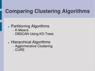
Categorization of Major Clustering Methods • Partitioning Methods • Density Based Methods • Grid Based Methods • Model Based Methods • Hierarchical Methods
Partitioning Methods • Given a database of n objects or data tuples, a partitioning method constructs k partitions of the data, where each partition represents a cluster and k≤n. • It classifies the data into k groups, which together satisfy the following requirements: • each group must contain at least one object, and • each object must belong to exactly one group. • Given k, the number of partitions to construct a partitioning method creates an initial partitioning. • It then uses an iterative relocation technique that attempts to improve the partitioning by moving objects from one group to another.
Density Based Methods • Most partitioning methods cluster objects based on the distance between objects. • Such methods can find only spherical-shaped clusters and encounter difficulty at discovering clusters of arbitrary density. • The idea is to continue growing the given cluster as long as the density (number of objects or data points) in the “neighborhood” exceeds some threshold. • DBSCAN and OPTICS are two density based methods.
Grid-Based Methods • Grid-based methods quantize the object space into a finite number of cells that form a gird structure. • All the clustering operations are performed on the grid structure. • The advantage of this approach is fast processing time • STING, CLIQUE, and Wave-Cluster are examples of grid-based clustering algorithms.
Model-based methods • Hypothesize a model for each of the clusters and find the best fit of the data to the given model. • A model-based algorithm may locate clusters by constructing a density function that reflects the spatial distribution of the data points.
Hierarchical Methods • Creates a hierarchical decomposition of the given set of data objects. • Two approaches: • agglomerative (bottom-up): starts with each object forming a separate group. Merges the objects or groups close to one another until all of the groups are merged into one, or until a termination condition holds. • divisive (top-down): starts with all the objects in the same cluster. In each iteration, a cluster is split up into smaller clusters, until eventually each object is one cluster, or until a termination condition holds. • This type of method suffers from the fact that once a step (merge or split) is done, it can never be undone. • BIRCH and CURE are examples of hierarchical methods.
BIRCH Balanced Iterative Reducing and Clustering Using Hierarchies • Begins by partitioning objects hierarchically using tree structures, and then applies other clustering algorithms to refine the clusters.
Clustering Problem • Given the desired number of cluster K and a dataset of N points, and a distance-based measurement function, we are asked to find a partition of the dataset that minimizes the value of the measurement function. • Due to an abundance of local minima, there is typically no way to find a global minimal solution without trying all possible partitions. • Constraint: The amount of memory available is limited (typically much smaller than the data set size) and we want to minimize the time required for I/O.
Previous Work • Probability-based approaches: • Typically make the assumption that probability distributions on separate attributes are statistically independent of each other. • Makes updating and storing the clusters very expensive. • Distance-based approaches: • Assume that all data points are given in advance and can be scanned frequently. • Ignore the fact that not all data points in the dataset are equally important with respect to the clustering purpose. • Are global methods. They inspect all data points or all current clusters equally no matter how close or far away they are.
Contributions of BIRCH • BIRCH is local (instead of global). Each clustering decision is made without scanning all data points or currently existing clusters. • BIRCH exploits the observation that the data space is usually not uniformly occupied, and therefore not every data point is equally important for clustering purposes. • BIRCH makes full use of available memory to derive the finest possible subclusters while minimizing I/O costs.
Centroid Diameter D Radius R Definitions • Given the centroids of two clusters and : • -The centroid Euclidian distance D0 -The centroid Manhattan distanceD1
Definitions (cont.) • Given N1 d-dimensional data points in a cluster: where i=1,2,…,N1, and N2 data points in another cluster: where j =N1+1, N1+2,…,N1+N2 • -Average inter-cluster distance D2 -Average intra-cluster distance D3 • -Variance increase distance D4
CF = (5, (16,30),(54,190)) (3,4) (2,6) (4,5) (4,7) (3,8) Clustering Feature • A Clustering Feature (CF) is a triple summarizing the information that we maintain about a cluster. • N is the number of data points in the cluster • is the linear sum of the N data points: • SS is the square sum of the N data points:
CF Additivity Theorem • Assume that and are the CF vectors of two disjoint clusters. Then the CF vector of th cluster that is formed by merging the two disjoint clusters is: • From the CF definition and additivity theorem, we know that the CF vectors of clusters can be stored and calculated incrementally as clusters are merged. • We can think of a cluster as a set of data points, but only the CF vector is stored as summary.
CF Tree • A CF tree is a height-balanced tree with two parameters: • Branching factor B • Threshold T • Each nonleaf node contains at most B entries of the form [CFi,childi] where i=1,2,…B. • childi is a pointer to its i-th child node • CFi is the CF of the sub-cluster represented by this child. • A leaf node contains at most L entries, each of the form [CFi] where i=1,2,…,L. • A leaf node also represents a cluster made up of all the subclusters represented by its entries. • All entries in a leaf node must satisfy a threshold value T: the diameter (or radius) has to be less than T.
Root CF1 CF2 CF3 CF6 B = 7 L = 6 child1 child2 child3 child6 Non-leaf node CF1 CF2 CF3 CF5 child1 child2 child3 child5 Leaf node Leaf node prev CF1 CF2 CF6 next prev CF1 CF2 CF4 next CF Tree
Insertion into a CF Tree • Given entry “Ent” • Identify the appropriate leaf: Starting from the root, it recursively descends the CF tree by choosing the closest child node according to a chosen distance metric: D0,D1,D2,D3 or D4 • Modify the leaf: When it reaches a leaf node, it finds the closest leaf entry, say Li and then tests whether Li can absorb “Ent” without violating the threshold condition. If so, the CF vector for Li is updated to reflect this. If not, an new entry for “Ent” is added to the leaf. If there is space on the leaf for this new entry, we are done, otherwise we must split the leaf node.
Insertion into a CF Tree (cont.) • Modify the path to the leaf: After inserting “Ent” into a leaf, we must update the CF information for each nonleaf entry on the path to the leaf. Without a split, this simply involves adding CF vectors to reflect the addition of “Ent”. A leaf split requires us to insert a new nonleaf entry into the parent node, to describe the newly created leaf. If the parent has space for this entry, at all higher levels, we only need to update the CF vectors to reflect the addition of “Ent”. In general, however, we may have to split the parent as well, and so up to the root. If the root I split, the tree height increases by one.
Performance of BIRCH • Tested on three datasets used as base Work load with D as the “weighted average diameter”. Each dataset consists of K clusters of 2-d data points. A cluster is characterized by the number of data points in it (n), its radius (r), and its center (c). • Running time is basically linear wrt N, and does not depend on the order (unlike CLARANS).
Performance • In conclusion, BIRCH uses much less memory, but is faster, more accurate, and less order-sensitive compared with CLARANS. BIRCH Clusters of DS1 CLARA Clusters of DS1 Actual Clusters of DS1 CLARANS Clusters of DS1
Application to Real Dataset • BIRCH used to filter real images • Two similar images of trees with a partly cloudy sky as he background, taken at two different wavelengths (512x1024 pixels each). • NIR: Near-infrared band • VIS: Visible wavelength band • Soil scientists recieve hundreds of such image pairs and try to first filter the trees from the background, and then filter the trees into sunlit leaves, shadows and branches for statistical analysis.
Application (cont.) • Applied BIRCH to the (NIT,VIS) value pairs for all pixels in an image. • Weighted equally: obtain 5 clusters • Very bright part of sky • Ordinary part of sky • Clouds • Sunlit leaves • Tree branches and shadows on the trees • Pulled out the part of the data corresponding to (5) and used BIRCH again. This time NIR was weighted 10 times heavier than VIS.
CURE: Clustering Using REpresentatives A Hierarchical Clustering Algorithm that Uses Partitioning
Partitional Clustering • Find k clusters optimizing some criterion: (for example, minimize the squared-error)
Hierarchical Clustering • Use nested partitions and tree structures • Agglomerative Hierarchical Clustering: • Initially each point is a distinct cluster • Repeated merge the closest clusters D_avg D_min
CURE • CURE: proposed by Guha, Rastogi & Shim, 1998 • A new hierarchical clustering algorithm that uses a fixed number of points as representatives (partition) • Centroid based approach: uses 1 pt to represent cluster => too little information … sensitive to data shapes • All point based approach: uses all points to cluster => too much information … sensitive to outliers • A constant number c of well scattered points in a cluster are chosen, and then shrunk toward the center of the cluster by a specified fraction alpha • The clusters with the closest pair of representative points are merged at each step • Stops when there are only k clusters left, where k can be specified
Six Steps in CURE Algorithm Draw Random Sample Partially Cluster Partitions Partition Sample Data Label Data In Disk Cluster Partial Clusters Eliminate Outliers
CURE’s Advantages • More accurate: • Adjusts well to geometry of non-spherical shapes. • Scales to large datasets • Less sensitive to outliers • More efficient: • Space complexity: O(n) • Time complexity: O(n2logn) (O(n2) if dimensionality of data points is small)
Feature: Random Sampling • Key idea: apply CURE to a random sample drawn from the data set rather than the entire data set. • Advantages: • Smaller size • Filtering outliers • Concerns: may miss out or incorrectly identify certain clusters! • Experimental results show that, with moderate sized random samples, we were able to obtain very good clusters.
Feature: Partitioning for Speedup • Partition the sample space into p partitions, each of size n/p. • Partially cluster each partition until the final number of clusters in each partition reduces to n/(pq). (q > 1) • Collect all partitions and run a second clustering pass on the n/p partial clusters • Tradeoff: sample size vs. accuracy
Feature: Labeling Data on Disk • Input is a randomly selected sample. • Have to assign the appropriate cluster labels to the remaining data points • Each data point is assigned to the cluster containing the representative point closest to it • Advantage: using multiple points enables CURE to correctly to distribute the data points when clusters are non-spherical or non-union
Feature: Outliers Handling • Random sampling filters out a majority of the outliers. • The remaining few outliers in the random sample are distributed all over the sample space and gets further isolated. • The clusters which are growing very slowly are identified and eliminated as outliers. • Use a second level pruning to eliminate merging-together outliers: outliers form very small clusters.
Experiments: Parameter Sensitivity Comparison with BIRCH Scale-up
Dataset Setup Experiment with data sets • Data set 1 contains one big and two small circles. • Data set 2 consists of 100 clusters with centers arranged in a grid pattern and data points in each cluster following a normal distribution with mean at the cluster center.
Sensitivity Experiment • CURE is very sensitive to its user-specified parameters. • Shrinking fraction alpha. • Sample size s • Number of representatives c
Shrinking Factor Alpha • Alpha < 0.2, reduces to the centroid-based algorithm • Alpha > 0.7, becomes similar to the all-points approach. • 0.2 – 0.7 is a good range for alpha
Random Sample Size • Tradeoff between random sample size and accuracy
Number of Representatives • For smaller values of c, the quality of clustering suffers. • For values of c greater than 10, CURE always found the right clusters.
CURE vs. BIRCH: quality of clustering • BIRCH cannot distinguish between the big and small clusters. • MST (all-point approach) merges the two ellipsoids. • CURE successfully discovers the clusters in Data set 1.
CURE vs. BIRCH: Execution Time • Run both on dataset2: • CURE execution time is always lower than BIRCH • Partitioning improves CURE’s running time by > 50% • As sample size goes up, CURE’s execution time only slightly increases due to fixed sample size
Conclusion • CURE and BIRCH are two hierarchical clustering algorithms • CURE adjusts well to clusters having non-spherical shapes and wide variances in size. • CURE can handle large databases efficiently.
Acknowledgement • Sudipto Guha, Rajeev Rastogi, Kyuseok Shim: CURE: An Efficient Clustering Algorithm for Large Databases. SIGMOD Conference 1998: 73-84 • Jiawei Han and Micheline Kamber, Data Mining: Concepts and Techniques, Morgan Kaufmann Publishers, 2000. • Tian Zhang, Raghu Ramakrishnan, Miron Livny: BIRCH: An Efficient Data Clustering Method for Very Large Databases. SIGMOD Conf. 1996: 103-114