Download
1 / 16
160 likes | 290 Views
Transformations, Z-scores, and Sampling. September 21, 2011. Changing the unit of measurement. Variables can be recorded in different units of measurement. Most often, one measurement unit is a linear transformation of another measurement unit: x new = a + bx.

E N D
Transformations, Z-scores, and Sampling September 21, 2011
Changing the unit of measurement Variables can be recorded in different units of measurement. Most often, one measurement unit is a linear transformation of another measurement unit: xnew = a + bx. Temperatures can be expressed in degrees Fahrenheit or degrees Celsius.TemperatureFahrenheit = 32 + (9/5)* TemperatureCelsius a + bx. Linear transformations do not change the basic shape of a distribution (skew, symmetry, multimodal). But they do change the measures of center and spread: • Multiplying each observation by a positive number bmultiplies both measures of center (mean, median) and spread (IQR, s) by b. • Adding the same number a (positive or negative) to each observation adds a to measures of center and to quartiles but it does not change measures of spread (IQR, s).
Density curves A density curve is a mathematical model of a distribution. The total area under the curve, by definition, is equal to 1, or 100%. The area under the curve for a range of values is the proportion of all observations for that range. Histogram of a sample with the smoothed, density curve describing theoretically the population.
Density curves come in any imaginable shape. Some are well known mathematically and others aren’t.
Median and mean of a density curve The medianof a density curve is the equal-areas point: the point that divides the area under the curve in half. The meanof a density curve is the balance point, at which the curve would balance if it were made of solid material. The median and mean are the same for a symmetric density curve. The mean of a skewed curve is pulled in the direction of the long tail.
Normal distributions Normal – or Gaussian – distributions are a family of symmetrical, bell-shaped density curves defined by a mean m (mu) and a standard deviation s (sigma) : N(m,s). x x e = 2.71828… The base of the natural logarithm π = pi = 3.14159…
A family of density curves Here, means are the same (m = 15) while standard deviations are different (s = 2, 4, and 6). Here, means are different (m = 10, 15, and 20) while standard deviations are the same (s = 3).
The 68-95-99.7% Rule for Normal Distributions • About 68% of all observations are within 1 standard deviation (s) of the mean (m). • About 95% of all observations are within 2 s of the mean m. • Almost all (99.7%) observations are within 3 s of the mean. Inflection point mean µ = 64.5 standard deviation s = 2.5 N(µ, s) = N(64.5, 2.5) Reminder: µ (mu) is the mean of the idealized curve, while is the mean of a sample. σ (sigma) is the standard deviation of the idealized curve, while s is the s.d. of a sample.
N(64.5, 2.5) N(0,1) => Standardized height (no units) The standard Normal distribution Because all Normal distributions share the same properties, we can standardize our data to transform any Normal curve N(m,s) into the standard Normal curve N(0,1). For each x we calculate a new value, z (called a z-score).
When x is 1 standard deviation larger than the mean, then z = 1. When x is 2 standard deviations larger than the mean, then z = 2. Standardizing: calculating z-scores A z-scoremeasures the number of standard deviations that a data value x is from the mean m. When x is larger than the mean, z is positive. When x is smaller than the mean, z is negative.
Ex. Women heights N(µ, s) = N(64.5, 2.5) Women’s heights follow the N(64.5”,2.5”) distribution. What percent of women are shorter than 67 inches tall (that’s 5’6”)? Area= ??? Area = ??? mean µ = 64.5" standard deviation s = 2.5" x (height) = 67" m = 64.5” x = 67” z = 0 z = 1 We calculate z, the standardized value of x: Because of the 68-95-99.7 rule, we can conclude that the percent of women shorter than 67” should be, approximately, .68 + half of (1 - .68) = .84 or 84%.
.0082 is the area under N(0,1) left of z = -2.40 0.0069 is the area under N(0,1) left of z = -2.46 .0080 is the area under N(0,1) left of z = -2.41 Using the standard Normal table Table A gives the area under the standard Normal curve to the left of any z value. (…)
Percent of women shorter than 67” For z = 1.00, the area under the standard Normal curve to the left of z is 0.8413. N(µ, s) = N(64.5”, 2.5”) Area ≈ 0.84 Conclusion: 84.13% of women are shorter than 67”. By subtraction, 1 - 0.8413, or 15.87% of women are taller than 67". Area ≈ 0.16 m = 64.5” x = 67” z = 1
area right of z = 1 - area left of z Tips on using Table A Because the Normal distribution is symmetrical, there are 2 ways that you can calculate the area under the standard Normal curve to the right of a z value. Area = 0.9901 Area = 0.0099 z = -2.33 area right of z = area left of -z
Tips on using Table A To calculate the area between 2 z- values, first get the area under N(0,1) to the left for each z-value from Table A. Then subtract the smaller area from the larger area. A common mistake made by students is to subtract both z values. But the Normal curve is not uniform. area between z1 and z2 = area left of z1 – area left of z2 The area under N(0,1) for a single value of z is zero. (Try calculating the area to the left of z minus that same area!)
The cool thing about working with normally distributed data is that we can manipulate it, and then find answers to questions that involve comparing seemingly non-comparable distributions. We do this by “standardizing” the data. All this involves is changing the scale so that the mean now = 0 and the standard deviation =1. If you do this to different distributions it makes them comparable. N(0,1)