Download
1 / 42
420 likes | 537 Views
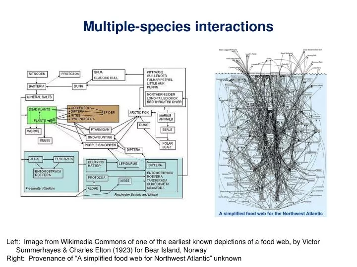
Multiple-species interactions. Left: Image from Wikimedia Commons of one of the earliest known depictions of a food web, by Victor Summerhayes & Charles Elton (1923) for Bear Island, Norway Right: Provenance of “A simplified food web for Northwest Atlantic” unknown. Food Webs.

E N D
Multiple-species interactions Left: Image from Wikimedia Commons of one of the earliest known depictions of a food web, by Victor Summerhayes & Charles Elton (1923) for Bear Island, Norway Right: Provenance of “A simplified food web for Northwest Atlantic” unknown
Food Webs Trophic (energy & nutrition) relationships among organisms Nodes Taxonomic or functional categories Links Flow of material (including energy-rich molecules) Paine, R. T. (1966) – Food webs are the “ecologically flexible scaffolding around which communities are assembled and structured” Provenance of image unknown
Food Webs Elton (1927) observed that predators tend to be larger & less numerous than their prey – “pyramid of numbers” (a.k.a. “Eltonian pyramid”) Elton’s hypothesis: Predators must be larger than prey to subdue them Pyramid could represent numbers, biomass, energy consumed per year, etc. Image from http://mrskingsbioweb.com/ecology.html
Food Webs Lindeman (1942) introduced the “energy-efficiency hypothesis” – the fraction of energy entering one trophic level that passes to the next higher level is low (~ 5 - 15%) The first and secondlawsofthermodynamics predict inefficiency: 1st Law = Conservation of Energy 2nd Law = Energy transformations result in an increase in entropy, i.e., only a fraction of the energy captured by one trophic level is available to do work in the next Inverted pyramids of biomass can occur (e.g., whales, krill, phytoplankton in southern oceans), but only when productivity and turnover of producers is extremely high
Food Webs Levin, S. A. (1992) – “Is a taxonomic subdivision most appropriate… would a functional one serve better? Should subdivision… consider different demographic classes, be partitioned according to genotype, etc.?” 2 Consumers “Green” or living food web Trophic levels within a simple food chain; donor levels supply energy or nutrients to recipient levels 1 Consumers 1 Producers 1 Consumers “Brown” or detrital food web 2 Consumers
Food Webs Web jargon: Connectance(c): Number of links (L) or connections between species (S) or nodes – expressed as a proportion of maximum connectance: c = L / [S(S-1)/2] Maximum connectance = S(S-1)/2 Linkage density(L/S): Average number of trophic links per species Compartmentation: Degree of isolation of subwebs – the number of species that interact with any given pair of species versus those that interact with only one member of the pair
Food Webs Web jargon: Omnivory: Feeding on more than one trophic level 4 4 Same-chain omnivory Different-chain omnivory 3’ 3 3 2’ 2 2 1’ 1 1
Food Webs Web jargon: Cycles & loops: Species have reciprocal feeding relationships Cycle E.g., wasps that prey on spiders that in turn catch wasps in their webs B A Loop E.g., “rock-paper-scissors” interactions among plankton (see Huisman refs.) B A C
Food Webs Modeling food webs: Which food web configurations promote stable equilibria? May (1973) and Pimm & Lawton (1977, 1978) used multispecies Lotka-Volterra models to examine various configurations for stability 4 0 = no connection / no interaction + = positive effect; prey supplying energy to predator - = negative effect; predation Values corresponded to interaction strengths 3 2 1
Food Webs Simulations generally examine the influence of small changes in predator & prey populations away from equilibria Two criteria for assessing stability: Do populations return to equilibrium sizes? How long does the system take to return to equilibrium? The way in which the matrices are constructed (e.g., lengths of food chains, connectedness, etc.) determines stability Do real-world food webs yield repeated patterns? If so, do the patterns have ecological significance?
Food Webs Are ratios of species at different trophic levels constant across communities? Cohen (1978) reviewed published community webs – relatively high consistency of predators to prey (4:3) This may simply reflect greater lumping into functional groups for prey than predators How long are food chains? As expected, relatively short; rarely more than 5 trophic levels (Pimm & Lawton 1977; Pimm 1982)
Food Webs How long are food chains? Yodzis (1984) – meta-analysis of 34 published food webs (Briand 1983) to examine the influence of energy efficiency on food-chain length Invertebrate ectotherms vs. vertebrate ectotherms vs. vertebrate endotherms at trophic level 2 Energy-conversion efficiency: invert. ectotherms > vert. ecototherms > vert. endotherms (invert. ectotherms are about an order of magnitude more efficient than vert. endotherms) Percent of chains supporting consumer(s): 23% > 9% > 6% invert. ectotherms > vert. ecototherms > vert. endotherms
Food Webs How long are food chains? Jenkins et al. (1992) – direct test of the energy-efficiency hypothesis If efficiency of energy transfer primarily determines food chain length, then manipulating productivity should influence food chain length Plastic buckets in an Australian forest to resemble water-filled tree-holes with different amounts of litter to generate a productivity gradient Natural tree-holes contain 4-level trophic chains: litter -- mosquito larvae -- larvae of predatory midge -- tadpoles Litter at 100% natural level (938 g/m2/yr), 10% natural level, 1% natural level Well-replicated study tracked for 48 wk
Food Webs How long are food chains? Jenkins et al. (1992) – direct test of the energy-efficiency hypothesis Decreased productivity resulted in decreased number of coexisting species & decreased number of trophic levels & links Figure from Jenkins et al. (1992)
Food Webs Modeling suggested that cycles, loops, and omnivory would destabilize food webs Do cycles and loops occur in nature? Is omnivory common? Polis (1991) – a skeptic of food web theory – characterized desert food webs in great detail Two-species cycles and three-species loops occur, and are especially common in communities characterized by size-dependent predation Role reversals between predators and prey are not uncommon Omnivory is quite common
Interaction Webs The distribution of interaction strengths is very important for determining modeling outcomes How are interaction strengths distributed in nature? Unlike the randomly defined interaction strengths of the earliest modeling approaches, interaction strengths are not normally distributed; they are heavily skewed toward weak interactions “…weak interactions may be the glue that binds natural communities together” (McCann, Hastings & Huxel 1998) This shows that evaluating interaction strength (of combined direct & indirect effects) and not merely trophic links is essential to understanding population dynamics and stability within food webs
Direct & Indirect Effects Dissecting exploitation competition reveals its indirect nature H H - - - + + P Solid arrows indicate direct effects, dotted arrows indicate indirect effects Redrawn from Menge (1995)
Direct & Indirect Effects Dissecting the ant-acacia mutualism reveals its indirect components H ant - - - + + + P As consumers, ants have direct negative effects on acacias (eating Beltian bodies, etc.), but indirect positive effects mediated through herbivores Solid arrows indicate direct effects, dotted arrow indicates indirect effect
Direct & Indirect Effects Tri-trophic Interaction or Trophic Cascade Apparent Competition C H - + - - + H + + + P P - - + P Solid arrows indicate direct effects, dotted arrows indicate indirect effects Redrawn from Menge (1995) & Morin (1999)
Direct & Indirect Effects Indirect Mutualism Keystone Predation Habitat Facilitation + H + H H H H - + - - - + + + • (e.g., inhibits feeding) + P P P P P - - Solid arrows indicate direct effects, dotted arrows indicate indirect effects Redrawn from Menge (1995) – found 83 distinct types of indirect interactions in 23 communities
Direct & Indirect Effects Interaction chain indirect effect – results from “linked direct interactions” (e.g., bird predators enhance barnacle abundance b/c they consume limpets that dislodge & sometimes consume barnacles); relatively predictable from the direct interactions bird barnacle limpet Interaction modification indirect effect – “a third species changes how a pair of species interacts;” the third species changes the per capita effect of one species on another (e.g., when barnacles are present, limpets are harder for birds to find); difficult to predict a priori bird barnacle limpet Figure modified from Wootton (1993)
Direct & Indirect Effects Density-mediated indirect interactions – “indirect effects… propagated by changes in densities of intervening species” e.g., “keystone predator effects, trophic cascades, and exploitative competition… [as] traditionally conceived” Approx. the same as interaction chain indirect effect Trait-mediated indirect interactions – “If a species reacts to the presence of a second species by altering its phenotype [phenotypic plasticity], the trait changes in the reacting species can alter the per capita effect of the reacting species on other species…” Approx. the same as interaction modification indirect effect Werner & Peacor (2003)
Direct & Indirect Effects Apparent competition (an example from Schmitt 1987) Prey species: Sessile bivalve filter feeders occur mostly in crevices Gastropods occur on rock surfaces and graze algae (Limited opportunities for direct competition, since neither diet nor space requirements overlap greatly) Common predators: Lobsters, octopi, whelks Apparent competition Experiment: Continually transplanted bivalves to maintain high densities of bivalves in sites with high densities of gastropods Prediction (if apparent competition operates): Predator density will increase, gastropod density will decrease C - - + + P P -
Direct & Indirect Effects Apparent competition (an example from Schmitt 1987) Found increased predator density and decreased gastropod density when bivalves were added relative to control sites Control sites Sites with added bivalves Figure modified from Schmitt (1987)
Direct & Indirect Effects How important are indirect effects? Menge (1995) reviewed 23 experimental studies of rocky intertidal habitats that were sufficiently well replicated and long enough in duration for indirect effects to become evident Considered only “ecologically significant” effects (that caused at least a 10% change in the abundance of one or more species) Found that 83 types of indirect effects accounted for 40% of the observed changes in community structure caused by manipulations (e.g., predator or prey removal) Most of the indirect effects were cases of keystone predation (35%) and apparent competition (25%) Exploitative competition constituted only 3% of indirect effects!
Bottom-Up vs. Top-Down Are abundances or distributions of organisms controlled by resources (bottom-up processes) or by predation & disease (top-down processes)? Trophic cascade Bottom-up view: Organisms at each trophic level are food limited Top-down view: Top level is food limited, lower levels are alternately predator vs. food limited (originated with Hairston, Smith & Slobodkin 1960 – HSS) C - + + H + - + P
Are Trophic Cascades “All Wet”? Polis (1991), Strong (1992) & etc. argued that the idea of discrete trophic levels, which trophic cascades are predicated on, is invalid b/c of the prevalence of omnivory Strong (1992) posed the question above, in part b/c omnivory appeared more prevalent in terrestrial communities (making trophic cascades more likely in aquatic communities) Photo of Gary Polis from http://science.marshall.edu/fet/euscorpius/images/polis.JPG
A Terrestrial Trophic Cascade A likely example of a terrestrial trophic cascade (McLaren & Peterson 1994) 500 km2 Isle Royale National Park in Lake Superior Primary producer: Balsam fir Herbivore: Moose (59% of winter diet is Balsam fir) Carnivore: Wolf (colonized island in 1959) Photo of Isle Royale from Wikipedia
A Terrestrial Trophic Cascade McLaren & Peterson (1994): “The shaded areas highlight intervals of forage suppression that… are closely tied to periods of elevated moose density, which in turn follow periods of low wolf density (note the lags…)… these intervals have no correspondence to AET [climatic fluctuations]” Figure from McLaren & Peterson (1994)
A Terrestrial Trophic Cascade A change in behavior of a top predator cascades through a community (Post et al. 1999) On Isle Royale, fluctuations in North Atlantic Oscillation (NAO) result in changes in winter snow accumulation Annual aerial surveys show close correlation between wolf pack size and the status of the NAO Photo of winter wolf pack (in Yellowstone National Park) from Wikipedia
A Terrestrial Trophic Cascade Post (1999): “a, Increase in the mean size of wolf packs in snowy (negative NAO) winters…” “b, Increase in the winter kill rate of wolf packs with pack size… kill rate per individual wolf also increased during snowy winters” “c, Decline in moose density one year after increase in size of winter wolf packs” “d, Increased growth of fir trees one year after decline in moose density” [notice reversed x-axis] Figure from Post (1999)
A Terrestrial Trophic Cascade Changes in wolf behavior have ecosystem-level effects on Isle Royale because moose dramatically influence net primary production, litter production & edaphic nutrient dynamics (Post et al. 1999) Photo of moose from Wikipedia
Bottom-Up vs. Top-Down Hunter and Price (1992) – we should always start with a bottom-up template: “the removal of higher trophic levels leaves lower levels present (if perhaps greatly modified), whereas the removal of primary producers leaves no system at all” Echoed in John McPhee’s (1998) Annals of the Former World, pg. 84: “Break the food chain and creatures die out above the link” Fretwell (1977) & Oksanen et al. (1981) – OFAN – proposed a reconciliation: productivity determines the number of trophic levels that can be supported in a community; plant productivity therefore ultimately dictates when top-down forces could cascade back down In general the top-down vs. bottom-up question applies to NPP, but in principal could be asked of a variety of variables at a variety of trophic levels.
Foundation Species Photo from Wikipedia; definitions from Ellison et al. (2005)
“Foundation Genotypes” Figure from Whitham et al. (2008)
Keystone Species Pisaster eating mussel Keystone predator – a predator whose activities maintain species diversity at lower trophic levels by disallowing competitive exclusion (Paine 1966) Barbet eating fig Keystone resource – first applied to plant species that sustain frugivores through periods of food scarcity in tropical forests, e.g., figs (Terborgh 1986) Photos from Wikipedia
Ecosystem Engineers Ecosytem engineer – an organism that creates, modifies, or maintains habitat (or microhabitat) by causing physical state changes in biotic or abiotic materials that, directly or indirectly, modulate the availability of resources to other species (Jones et al. 1994) An ecosystem engineer has a large impact beyond simply assimilating and dissimilating material The definition is especially useful when applied to organisms that modify the environment through means other than trophic activities Photo of Clive Jones from Cary Institute of Ecosystem Studies
Ecosystem Engineers Allogenic ecosystem engineer – organism that changes the environment by transforming living or nonliving materials from one physical state to another, via mechanical or other means (Jones et al. 1994) E.g., Beaver Photo of beaver dam on Tierra del Fuego from Wikipedia
Ecosystem Engineers Autogenic ecosystem engineer – organism that changes the environment via its own physical structures, i.e., living & dead tissues (Jones et al. 1994) E.g., Long-leaf pines K. Harms’ photo of Pinus palustris at Camp Whispering Pines, Tangipahoa Parish, LA
Assembly Rules Diamond (1975) coined the term for broad patterns of bird species distributions in the Bismark Archipelago & Solomon Islands Wilson & Whittaker (1995; pg. 801): “generalised restrictions on species presence or absence that are based on the presence or absence of one or several other species, or types of species (not simply the response of individual species to the environment)…” Connor & Simberloff (1979) kicked off a long and continuing debate about assembly rules and testing for them E. Weiher (quoted in Stokstad’s piece in Science, 2009, v. 326, pg. 34): “I think what we’re going to find out is that assembly rules are vague, gentle constraints” Photo of Jared Diamond from Wikipedia
Priority Effects Petraitis et al. (2009) provide an experimental example of priority effects and multiple stable statesin the Gulf of Maine Ice scour can create open patches; experiments mimicked these disturbances (rockweed stands cleared in 1996 and followed through 2005) In sheltered bays, rockweed stands or mussel beds established, depending on which arrived first, and were not invaded by the other species As required by Peterson (1984) to establish multiple stable states, “the very same site could come to be occupied by different, self-replicating communities” Figure from Petraitis et al. (2009)
Community Assembly / Coalescence “We use the term community coalescence to refer to the development of complex ecological communities from a regional species pool. This coalescence depends on interactions among species availability, physical environment, evolutionary history, and temporal sequence of assembly.” From: J. N. Thompson et al. 2001. Frontiers of Ecology. BioScience 51:15-24.