Download
1 / 12
120 likes | 231 Views
Data Analysis Algorithm for GRB triggered Burst Search. Soumya D. Mohanty Center for Gravitational Wave Astronomy University of Texas at Brownsville On behalf of the External Triggers Subgroup of the LSC Bursts Upper Limit group. Summary.

E N D
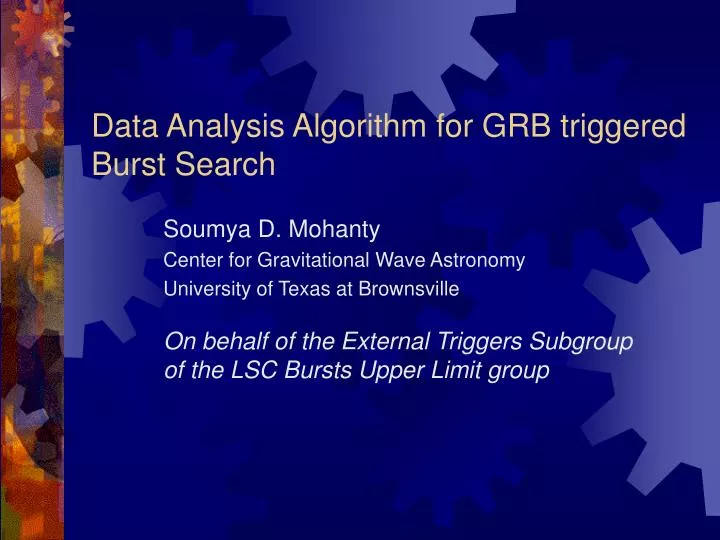
Data Analysis Algorithm for GRB triggered Burst Search Soumya D. Mohanty Center for Gravitational Wave Astronomy University of Texas at Brownsville On behalf of the External Triggers Subgroup of the LSC Bursts Upper Limit group
Summary • Presents details of the search algorithm developed by the external triggers subgroup for a GRB triggered search • Applied to GRB030329 (results presented by Marka) • Aim of the algorithm : Deep search in a short time segment around one GRB trigger • Must be robust against non-Gaussianity and non-stationarity • Basic ideas and first version of the algorithm presented at AMALDI’03 • Significant improvements since then • More background details in a series of LIGO technical notes GWDAW 2003
Specifications for the algorithm • GW Burst waveform unknown • Multiple IFOs • Offset between GRB and GWB unknown but bounded by astrophysical models ( of order ~10 sec) • GWB duration expected to be of order ~ 10 msec • Long signals possible (van Putten) and searched for (Marka) but not included in this talk GWDAW 2003
Why cross-correlation? Non-Gaussian Non-Gaussian noise : x1, x2 performance may exceed(x1,x2) • Cross-correlation is intuitive but is there a deeper justification? • A frequentist approach for a simple case : What is the Maximum Likelihood Ratio test ? • Stationary Gaussian white noise • Pair of independent identical colocated colaligned detectors • Unknown signal waveform • (x1,x2) = maxh p(x1,x2|h) / p(x1,x2 |0) • Signal parameters : signal samples h[k] • x, y = k x[k] y[k] • (x1,x2) = x1, x1 /4 + x2, x2 /4 + x1, x2 /2 GWDAW 2003
Properties of Cross-correlation • Free parameters : offset from trigger, integration length • Optimum Integration length for a given signal • Depends on signal duration and amplitude (quadratic) • Even if signal duration were known a priori, a range of integration lengths must be used for signal detection • Parameter scan required over ( at least ) offset and integration length • Sensitive to non-stationarity in rms. Options : • Use Pearson’s correlation coefficient (normalize with variance of the same data segments) OR • Use local “off-source” data for standardization • Sensitive to the presence of lines • Data Conditioning required GWDAW 2003
GRB030329 • Data Conditioning • Bandpass filtering (100 to 2000 Hz) • LPC trained on a short section of neighbouring data (Chatterjee) • Output: approximately whitened data • Applicable to any GRB • H1 and H2 were in lock so no direction dependent time shifts needed • Required in the general case • TAMA also in lock (work in progress) GWDAW 2003
Parameter scan : basic idea • Parameters : Offset from trigger and integration length • Result of scan : CORRGRAM • 2D plane • Each pixel is the cross-correlation value for a given offset and integration length • Detect signals via identification of clusters of “high significance” pixels GWDAW 2003
Modifications • Max signal response will not occur at exactly 0 time shift • Combine cross-correlation values time shifts around 0 • Construct cross-correlation sequences C12[k] and C21[k] • Mutually independent IFO data C12[k] and C21[k] independent sum in quadrature C[k]2=C12[k]2+C21[k]2 • Important : C[k] generated for each point in the offset, integration length grid GWDAW 2003
Standardization • Estimate noise only variance and mean from C[k] ; k >> Integration length (“lobes”) • Standardize C[k] ; k ~ integration length (“core”) • Sum standardized “core” samples • Standardization makes the algorithm more robust to rms fluctuations while preventing signal saturation C[k] Lag GWDAW 2003
Estimation of pixel significance • Each pixel of corrgram now is a sum of cross-correlations over nearby time shifts rather than just shift=0 • Different integration lengths lead to different marginal densities for pixel values • Marginal distribution estimated from pixel values over all offset for a fixed integration length with outlier trimming (top 1%) GWDAW 2003
Final steps • Threshold (low) on significance • With respect to estimated marginal density • Identify cluster of 5 adjacent pixels • Group clusters separated by < 65 msec • Find average of five loudest pixels in each cluster • Threshold • Performance characterization via signal injections already discussed GWDAW 2003
Plans • Alternative conditioning schemes to be tested • MBLT, MNFT, Coherent line removal, Kalman filter • Apply pipeline to more S2+DT8 / S3 GRBs • Generalize to > 2 detectors • Generalize to quasi-monochromatic signals • Refinements to algorithm and simulations • Modeled data playground GWDAW 2003