Download

1 / 28
280 likes | 283 Views
(Generalized) Mixed-Effects Models – (G)MEMs. Yann Hautier, NutNet meeting 16 th Aug 2011. MEM. Maximum Entropy Models (Grace 2011). MEM. Maximum Entropy Models (Grace 2011) Muddled Eric Models (Seabloom 2011). MEM. Maximum Entropy Models (Grace 2011) Muddled Eric Models (Seabloom 2011)

E N D
(Generalized) Mixed-Effects Models – (G)MEMs Yann Hautier, NutNet meeting 16th Aug 2011
MEM Maximum Entropy Models (Grace 2011)
MEM Maximum Entropy Models (Grace 2011) Muddled Eric Models (Seabloom 2011)
MEM Maximum Entropy Models (Grace 2011) Muddled Eric Models (Seabloom 2011) Mixed-Effects Models (Fischer 1918)
MEM – Maximum Mikelihood Given a set of data and a chosen model which parameters of the model produce the best model fit and make the data most likely to be observed
Fixed and Random Effects Fixed effects: Experimentally manipulated factors Influence only the mean of a response BLUEs (Best Linear Unbiased Estimates) Unknown constants to be estimated from data Limited to the range of the fixed effect examined Random effects Blocks, Plots, Sites, etc.; random subset of larger population Influence the variance/covariance structure BLUPs (Best Linear Unbiased Predictions) ‘Prediction’ of the population of random effects
Fixed and Random Effects Fixed effects: Experimentally manipulated factors Influence only the mean of a response BLUEs (Best Linear Unbiased Estimates) Unknown constants to be estimated from data Limited to the range of the fixed effect examined Random effects Blocks, Plots, Sites, etc.; random subset of larger population Influence the variance/covariance structure BLUPs (Best Linear Unbiased Predictions) ‘Prediction’ of the population of random effects Not inequivocal – grey area in between
Why use mixed-effects models? • To properly account for covariance structure in grouped data • To treat fixed and random effects appropriately • Fixed effects: Estimate and test • Random effects: Predict and test
Why use Modern Mixed-effects Models (in particular)? • Modern methods (ML, REML etc.) can give unbiased predictions of variance components for unbalanced data • More efficient use of degrees of freedom than traditional approach because fixed x random interactions are random terms and only require 1 DF to estimate VC • Estimating variance components by ML-based method avoids the mixed-model debate over correct error term since the VCs are estimated directly by REML etc. • To get shrinkage estimates and reduce risk of over-fitting • To properly account for covariance structure in grouped data
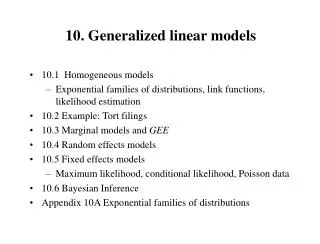
Generalized Linear Mixed Models (GLMMs) • Combine the properties of two statistical frameworks • Linear mixed models (incorporation random effects) • Generalized linear models (handling non normal data by using link functions and exponential family)
lm, lme, lmer syntax lm(X ~ Y, data) lme(X ~ Y, random = list(Site = ~1 + sr.log2, Block = ~1, mix = ~1), data) lmer(X ~ Y + (1 + logS | site) + (1| Block ) + (1| mix), family = " ", data) Family: binomial(link = "logit") gaussian(link = "identity") Gamma(link = "inverse") inverse.gaussian(link = "1/mu^2") poisson(link = "log") quasi(link = "identity", variance = "constant") quasibinomial(link = "logit") quasipoisson(link = "log")
Example – MachinesBalanced vs. Unbalanced data ls1Machine <- lme( score ~ Machine, data = Machines) (Intercept) MachineB MachineC 52.355556 7.966667 13.916667 delete selected rows from the Machines data MachinesUnbal <- Machines[ -c(2,3,6,8,9,12,19,20,27,33), ] ls2Machine <- lme( score ~ Machine, data = MachinesUnbal) (Intercept) MachineB MachineC 52.321028.0083713.95120
Example – MachinesBalanced vs. Unbalanced data fm1Machine <- lme( score ~ Machine, data = Machines, random = ~ 1 | Worker / Machine) (Intercept) MachineB MachineC 52.355556 7.966667 13.916667 delete selected rows from the Machines data MachinesUnbal <- Machines[ -c(2,3,6,8,9,12,19,20,27,33), ] fm2Machine <- lme( score ~ Machine, data = MachinesUnbal , random = ~ 1 | Worker / Machine) (Intercept) MachineB MachineC 52.354000 7.962446 13.918222
Example – BIODEPTH Manipulation of diversity: Species richness Species composition Hector et al. 1999, Science
Example – BIODEPTHDegrees of freedom ls1 <- lm(terms(ANPP~ Site+Block+SR.log2+Site:SR.log2+Mix+Site:Mix, keep.order= TRUE), data= Biodepth) Df Sum Sq Mean Sq F value Pr(>F) Site 7 14287153 2041022 126.5168 < 2.2e-16 *** Block 7 273541 39077 2.4223 0.02072 * SR.log2 1 5033290 5033290 311.9986 < 2.2e-16 *** Site:SR.log2 7 1118255 159751 9.9025 9.316e-11 *** Mix 189 17096361 90457 5.6072 < 2.2e-16 *** Site:Mix 28 1665935 59498 3.6881 2.252e-08 *** Residuals 224 3613660 16132 mem1 <- lmer(ANPP~ SR.log2 +(1|Site)+(1|Block)+(1|Mix)+(1|Site:Mix), data= Biodepth) Df Sum Sq Mean Sq F value SR.log2 1 772347 772347 47.544
Example – BIODEPTHDegrees of freedom ls1 <- lm(terms(ANPP~ Site+Block+SR.log2+Site:SR.log2+Mix+Site:Mix, keep.order= TRUE), data= Biodepth) Df Sum Sq Mean Sq F value Pr(>F) Site 7 14287153 2041022 126.5168 < 2.2e-16 *** Block 7 273541 39077 2.4223 0.02072 * SR.log2 1 5033290 5033290 311.9986 < 2.2e-16 *** Site:SR.log2 7 1118255 159751 9.9025 9.316e-11 *** Mix 189 17096361 90457 5.6072 < 2.2e-16 *** Site:Mix 28 1665935 59498 3.6881 2.252e-08 *** Residuals 224 3613660 16132 mem1 <- lmer(ANPP~ SR.log2 +(1|Site)+(1|Block)+(1|Mix), data= Biodepth) mem2 <- lmer(ANPP~ SR.log2 +(1|Site)+(1|Block), data= Biodepth) Df AIC BIC logLik Chisq Chi Df Pr(>Chisq) mem2 5 6394.7 6415.4 -3192.4 mem1 6 6277.3 6302.1 -3132.6 119.41 1 < 2.2e-16 *** Uses only 6 DF instead of 7+7+1+7+189+28=239!!!
Example – BIODEPTHError terms Spehn et al. 2005
Example – BIODEPTHError terms Spehn et al. 2005
Example – BIODEPTHError terms mem3 <- lme (ANPP~ SR.log2+Site, random=list(Block = ~1, Mix = ~1), data= Biodepth, na.action=na.omit) numDF denDF F-value p-value (Intercept) 1 413 1781.8981 <.0001 SR.log2 1 413 94.3233 <.0001 Site 7 7 33.4856 1e-04 mem4 <- lme (ANPP~ SR.log2+Block, random=list(Site = ~1, Mix = ~1), data= Biodepth, na.action=na.omit) numDF denDF F-value p-value (Intercept) 1 224 457.6593 <.0001 SR.log2 1 224 57.2133 <.0001 Block 7 217 6.0297 <.0001 Crossed-random effects – to be considered with care. Not handled by lme, lmer would do the job, but no P-values!!!
Crossed random effects Block Species compossition
Shrinkage No pooling (lmList(ANPP~ SR.log2|Site, data= Biodepth))
Shrinkage No pooling (lmList(ANPP~ SR.log2|Site, data= Biodepth)) Complete pooling (lm(ANPP~ SR.log2, data= Biodepth))
Shrinkage No pooling (lmList(ANPP~ SR.log2|Site, data= Biodepth)) Complete pooling (lm(ANPP~ SR.log2, data= Biodepth)) Mixed-effects models (lmer(ANPP~ SR.log2 +(SR.log2|Site)+(1|Block)+(1|Mix)+(1|Site:Mix), data= Biodepth))
Mixed-effects model analysis: Overview • Estimate and test the fixed effects just as in fixed-effects analysis but it makes no sense to estimate and test the random effects. • Instead the random effects are treated as in variance components analysis: we predict and test the variance components (often expressed in standard deviation form so that they are back on the original scale of the response). • The covariances (or correlations) between random effects can also be estimated – between repeated measurement locations or times for example • Fixed effects and random effects are tested differently.