Download
1 / 31
350 likes | 1.69k Views
Introduction to Precipitation . CEE 4420 – Engineering Hydrology (Prepared by Abebe Gebregiorgis). 2.1 Introduction . All forms of water that reach the earth from the atmosphere is called Precipitation .

E N D
Introduction to Precipitation CEE 4420 – Engineering Hydrology (Prepared by Abebe Gebregiorgis)
2.1 Introduction • All forms of water that reach the earth from the atmosphere is called Precipitation. • The usual forms are rainfall, snowfall, frost, hail, dew. Of all these, the first two contribute significant amounts of water. • Rainfall being the predominant form of precipitation causing stream flow, especially the flood flow in majority of rivers. Thus, in this context, rainfall is used synonymously with precipitation.
Introduction…. • In nature water is present in three aggregation states: • solid: snow and ice; • liquid: pure water and solutions; • gaseous: vapors under different grades of pressure and saturation • The water exists in the atmosphere in these three aggregation states.
Introduction…. • Types of precipitation • Rain, snow, hail, drizzle, glaze, sleet • Rain: • Is precipitation in the form of water drops of size larger than 0.5 mm to 6mm • The rainfall is classified in to • Light rain – if intensity is trace to 2.5 mm/h • Moderate – if intensity is 2.5 mm/hr to 7.5 mm/hr • Heavy rain – above 7.5 mm/hr
Introduction…. • Snow: • Snow is formed from ice crystal masses, which usually combine to form flakes • Hail (violent thunderstorm) • precipitation in the form of small balls or lumps usually consisting of concentric layers of clear ice and compact snow. • Hail varies from 0.5 to 5 cm in diameter and can be damaging crops and small buildings.
2.2 Temporal and Spatial Variation of Rainfall • Rainfall varies greatly both in time and space • With respect to time – temporal variation • With space – Spatial variation • The temporal variation may be defined as hourly, daily, monthly, seasonal variations and annual variation (long-term variation of precipitation)
2.3. Measurement of Rainfall • Rainfall and other forms of precipitation are measured in terms of depth, the values being expressed in millimeters. • One millimeter of precipitation represents the quantity of water needed to cover the land with a 1mm layer of water, taking into account that nothing is lost through drainage, evaporation or absorption. • Instrument used to collect and measure the precipitation is called raingauge.
Rainfall measurement… Precipitation gauge 1 - pole 2 - collector 3 - support- galvanized metal sheet 4 – funnel 5 - steel ring 1. Non recording gauge
2. Recording gauge / graphic raingauge • The instrument records the graphical variation of the fallen precipitation, the total fallen quantity in a certain time interval and the intensity of the rainfall (mm/hour). • It allows continuous measurement of the rainfall. The graphic rain gauge 1-receiver 2-floater 3-siphon 4-recording needle5-drum with diagram 6-clock mechanism
3. Tele-rain gauge with tilting baskets • The tele-rain gauge is used to transmit measurements of precipitation through electric or radio signals. • The sensor device consists of a system with two tilting baskets, which fill alternatively with water from the collecting funnel, establishing the electric contact. • The number of tilting is proportional to the quantity of precipitation hp
Tele-rain gauge …… The tele-rain-gauge 1 - collecting funnel 2 - tilting baskets 3 - electric signal 4 - evacuation
4. Radar measurement of rainfall • The meteorological radar is the powerful instrument for measuring the area extent, location and movement of rainstorm. • The amount of rainfall overlarge area can be determined through the radar with a good degree of accuracy • The radar emits a regular succession of pulse of electromagnetic radiation in a narrow beam so that when the raindrops intercept a radar beam, its intensity can easily be known.
Raingauge Network • Since the catching area of the raingauge is very small as compared to the areal extent of the storm, to get representative picture of a storm over a catchment the number of raingauges should be as large as possible, i.e. the catchment area per gauge should be small. • There are several factors to be considered to restrict the number of gauge: • Like economic considerations to a large extent • Topographic & accessibility to some extent.
Raingauge Network….. • World Meteorological Organization (WMO) recommendation: • In flat regions of temperate, Mediterranean and tropical zones • Ideal 1 station for 600 – 900 km2 • Acceptable 1 station for 900 – 3000 km2 • In mountainous regions of temperate , Mediterranean and tropical zones • Ideal 1 station for 100 – 250 km2 • Acceptable 1 station for 250 – 1000 km2 • In arid and polar zone • 1 station for 1500 – 10,000 km2 • 10 % of the raingauges should be self recording to know the intensity of the rainfall
2.4 Preparation of Data • Before using rainfall data, it is necessary to check the data for continuing and consistency • Missing data • Record errors Estimation of Missing Data • Given annual precipitation values – P1, P2, P3,… Pm at neighboring M stations of station X 1, 2, 3 & m respectively • The normal annual precipitation given by N1, N2, N3,…, Nm, Ni… (including station X) • To find the missing precipitation, Px , of station X
Test for consistency record (Double mass curve techniques) • Let a group of 5 to 10 base stations in the neighbourhood of the problem station X is selected • Arrange the data of X stn rainfall and the average of the neighbouring stations in reverse chronological order (from recent to old record) • Accumulate the precipitation of station X and the average values of the group base stations starting from the latest record. • Plot the against as shown on the next figure • A decided break in the slope of the resulting plot is observed that indicates a change in precipitation regime of station X, i.e inconsistency. • Therefore, is should be corrected by the factor shon on the next slide
Test for consistency record…. a c Pcx – corrected precipitation at any time period t1 at stationX Px – Original recorded precp. at time period t1 at station X Mc – corrected slope of the double mass curve Ma – original slope of the mass curve
2.5 Mean Precipitation over an area • Raingauges rainfall represent only point sampling of the areal distribution of a storm • The important rainfall for hydrological analysis is a rainfall over an area, such as over the catchment • To convert the point rainfall values at various stations to in to average value over a catchment, the following methods are used: • arithmetic mean • the method of the Thiessen polygons • the isohyets method
Arithmetic Mean Method • When the area is physically and climatically homogenous and the required accuracy is small, the average rainfall ( ) for a basin can be obtained as the arithmetic mean of the hi values recorded at various stations. • Applicable rarely for practical purpose
Method of Thiessen polygons • The method of Thiessen polygons consists of attributing to each station an influence zone in which it is considered that the rainfall is equivalent to that of the station. • The influence zones are represented by convex polygons. • These polygons are obtained using the mediators of the segments which link each station to the closest neighbouring stations
Thiessen polygons ………. P7 P6 A7 A6 P2 A2 A1 A8 A5 P1 P8 P5 A4 A3 P3 P4
Thiessen polygons ………. Generally for M station The ratio is called the weightage factor of station i
Isohyetal Method • An isohyet is a line joining points of equal rainfall magnitude. 10.0 8 D a5 6 C 12 9.2 12 a4 a3 7.0 B 4 7.2 A E a2 10.0 9.1 4.0 a1 a1 F 8 6 4
Isohyetal Method • P1, P2, P3, …. , Pn – the values of the isohytes • a1, a2, a3, …., a4 – are the inter isohytes area respectively • A – the total catchment area • - the mean precipitation over the catchment NOTE The isohyet method is superior to the other two methods especially when the stations are large in number.
2.6 Intensity – Duration – Frequency (IDF) Relationship Mass Curve of Rainfall 1st storm, 16 mm 2nd storm, 16 mm
Hyetograph IDF …. • is a plot of the accumulated precipitation against time, plotted in chronological order Total depth = 10.6 cm Duration = 46 hr
IDF …. • In many design problems related to watershed such as runoff disposal, erosion control, highway construction, culvert design, it is necessary to know the rainfall intensities of different durations and different return periods. • The curve that shows the inter-dependency between i (cm/hr), D (hour) and T (year) is called IDF curve. • The relation can be expressed in general form as: i – Intensity (cm/hr) D – Duration (hours) K, x, a, n – are constant for a given catchment
IDF …. k = 6.93 x = 0.189 a = 0.5 n = 0.878