Download
1 / 91
950 likes | 2.19k Views
7 th Iranian Workshop on Chemometrics 3-5 February 2008. Initial estimates for MCR-ALS method: EFA and SIMPLISMA. Bahram Hemmateenejad Chemistry Department, Shiraz University, Shiraz, Iran E-mail: hemmatb@sums.ac.ir. Chemical modeling. Fitting data to model (Hard model)

E N D
7th Iranian Workshop on Chemometrics 3-5 February 2008 Initial estimates for MCR-ALS method: EFA and SIMPLISMA Bahram Hemmateenejad Chemistry Department, Shiraz University, Shiraz, Iran E-mail: hemmatb@sums.ac.ir
Chemical modeling Fitting data to model (Hard model) Fitting model to data (soft model)
Goal: Given an I x J matrix, D, of N species, determine N and the pure spectra of each specie. Model: DIxJ = CIxNSNxJ Common assumptions: Non-negative spectra and concentrations Unimodal concentrations Kinetic profiles 1 0.5 = S N x J 0 30 60 20 C 40 10 20 I x N 0 0 samples sensors D I x J Multicomponent Curve Resolution
Basic Principles of MCR methods PCA: D=TP Beer-Lambert: D=CS In MCR we want to reach from PCA to Beer-Lambert • D= TP = TRR-1P, R: rotation matrix • D = (TR)(R-1P) • C=TR, S=R-1P • The critical step is calculation of R
Multivariate Curve Resolution-Alternative Least Squares (MCR-ALS) • Developed by R. Tauler and A. de Juan • Fully soft modeling method • Chemical and physical constraints • Data augmentation • Combined hard model • Tauler R, Kowalski B, Fleming S, ANALYTICAL CHEMISTRY 65 (15): 2040-2047, 1993. • de Juan A, Tauler R, CRITICAL REVIEWS IN ANALYTICAL CHEMISTRY 36 (3-4): 163-176 2006
MCR-ALS Theory • Widely Applied to spectroscopic methods • UV/Vis. Absorbance spectra • UV-Vis. Luminescence spectra • Vibration Spectra • NMR spectra • Circular Dichroism • … • Electrochemical data are also analyzed
MCR-ALS Theory • In the case of spectroscopic data • Beer-Lambert Law for a mixture • D(mn) absorbance data of k absorbing species D = CS • C(mk) concentration profile • S(kn) pure spectra
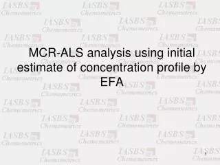
MCR-ALS Theory • Initial estimate of C or S • Evolving Factor Analysis (EFA) C • Simple-to-use Interactive Self-Modeling Mixture Analysis (SIMPLISMA) S
MCR-ALS Theory • Consider we have initial estimate of C (Cint) • Determination of the chemical rank • Least square solution for S: S=Cint+ D • Least square solution for C: C=DS+ • Reproducing of Dc: Dc=CS • Calculating lack of fit error (LOF) Go to step 2
Constraints in MCR-ALS • Non-negativity (non-zero concentrations and absorbencies) • Unimodality (unimodal concentration profiles). Its rarely applied to pure spectra • Closure (the law of mass conservation or mass balance equation for a closed system) • Selectivity in concentration profiles (if some selective zooms are available) • Selectivity in pure spectra (if the pure spectra of a chemical species, i.e. reactant or product, are known)
Constraints in MCR-ALS • Peak shape constraint • Hard model constraint (combined hard model MCR-ALS)
Rotational Ambiguity • Rank Deficiency
Evolving Factor Analysis(EFA) • Gives a raw estimate of concentration profiles • Repeated Factor analysis on evolving submatrices • Gampp H, Maeder M, Meyer CI, Zuberbuhler AD, CHIMIA 39 (10): 315-317 1985 • Maeder M, Zuberbuhler AD, ANALYTICA CHIMICA ACTA 181: 287-291, 1986 • Gampp H, Maeder M, Meyer CJ, Zuberbuhler AD, TALANTA 33 (12): 943-951, 1986
Basic EFA ExampleCalculate Forward Singular Values 1 ___ 1st Singular Value 1 0.9 ----- 2nd Singular Value SVD ...… 3rd Singular Value 0.8 S 0.7 i R 0.6 i 0.5 0.4 0.3 0.2 0.1 I 0 0 5 10 15 20 25 I samples
Basic EFA ExampleCalculate Backward Singular Values 1 1 ___ 1st Singular Value 0.9 ----- 2nd Singular Value 0.8 ...… 3rd Singular Value 0.7 R 0.6 0.5 0.4 i SVD 0.3 S 0.2 i 0.1 I 0 0 5 10 15 20 25 I samples
Basic EFA • Use ‘forward’ and ‘backward’ singular values to estimate initial concentration profiles • Area under both nth forward and (K-n+1)th backward singular values is estimate for initial concentration of nth component. 1 0.9 0.8 0.7 0.6 0.5 0.4 0.3 0.2 0.1 0 0 5 10 15 20 25 I samples
1 0.9 0.8 0.7 0.6 0.5 0.4 0.3 0.2 0.1 0 0 5 10 15 20 25 samples I Basic EFA First estimated spectra Area under 1st forward and 3rd backward singular value plot. (Blue) Compare to true component (Black)
1 0.9 0.8 0.7 0.6 0.5 0.4 0.3 0.2 0.1 0 0 5 10 15 20 25 I samples Basic EFA First estimated spectra Area under 2nd forward and 2nd backward singular value plot. (Red) Compare to true component (Black)
1 0.9 0.8 0.7 0.6 0.5 0.4 0.3 0.2 0.1 0 0 5 10 15 20 25 I samples Basic EFA First estimated spectra Area under 3rd forward and 1st backward singular value plot. (Green) Compare to true component (Black)
Example data • Spectrophotometric monitoring of the kinetic of a consecutive first order reaction of the form of A B C k1 k2
Pseudo first-order reaction with respect to A • A + R B C • [R]1 k1=0.20 k2=0.02 • [R]2 k1=0.30 k2=0.08 • [R]3 k1=0.45 k2=0.32 k1 k2
K1=0.2 K2=0.02 K1=0.3 K2=0.08 K1=0.45 K2=0.32
K1=0.30 K2=0.08 K1=0.20 K2=0.02 K1=0.45 K2=0.32
EFA Analysis • The m.file is downloadable from the MCR-ALS home page: http://www.ub.edu/mcr/welcome.html