Download
1 / 32
320 likes | 492 Views
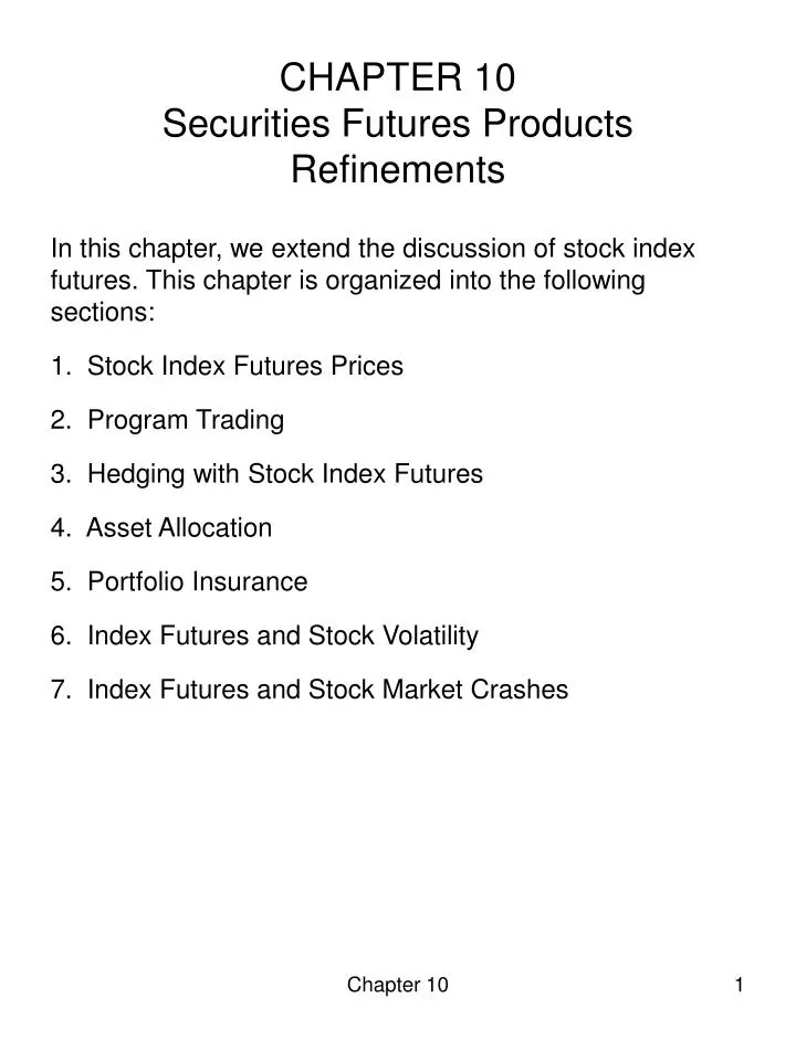
CHAPTER 10 Securities Futures Products Refinements. In this chapter, we extend the discussion of stock index futures. This chapter is organized into the following sections: Stock Index Futures Prices Program Trading Hedging with Stock Index Futures Asset Allocation

E N D
CHAPTER 10Securities Futures Products Refinements • In this chapter, we extend the discussion of stock index futures. This chapter is organized into the following sections: • Stock Index Futures Prices • Program Trading • Hedging with Stock Index Futures • Asset Allocation • Portfolio Insurance • Index Futures and Stock Volatility • Index Futures and Stock Market Crashes Chapter 10
Stick Index Futures Prices • In this section, the following issues are explored: • The empirical evidence on stock index futures efficiency. • do stock index futures prices conform to the Cost-of-Carry Model? • The effect of taxes on stock index futures prices. • The timing relationship between stock index futures prices and the cash market index. • Does the futures price lead the cash market index, or does the cash market index lead the futures? • The seasonal impacts on stock index futures pricing. Chapter 10
Stock Index Futures Efficiency • Recall that the success of an arbitrage opportunity can be affected by: • The use of short sale proceeds • Transaction costs • Dividend variability • Every real market has a range of permissible no-arbitrage prices. This no-arbitrage band increases because of transaction costs and restrictions on short selling. • Evidence suggests that the futures market was inefficient in the early days of trading but now it conforms well to the Cost-of-Carry Model. • Figure 10.1 shows the result of a study by Modest and Sundaresan. Chapter 10
Stock Index Futures Efficiency • Insert figure 10.1 here • Notice how the observed price is almost always within the no arbitrage bounds and never deviates far from them. Chapter 10
Effect of Taxes on Stock Index Futures Prices • Because futures prices are marked-to-market at year end for tax purposes, index futures contracts possess no tax-timing options. In the futures markets, tax rules require all paper gains or losses to be recognized as cash gains or losses each year. In the cash market, an individual can time his tax gains or losses. • In an empirical study of the effect of the tax-timing option, Cornell concludes that the tax-timing option does not appear to affect prices. Chapter 10
Timing Effect on Stock Index Futures Prices • The Day of the Week Effect in Stock Index Futures • A great deal of evidence shows that returns on stocks differ depending on the day of the week. In particular, Friday returns are generally high. • Leads and Lags in Stock Index Prices • Leads and lags in stocks index prices refer to which market drives the other. • Does the futures price lead the cash market index, or does the cash market index lead the futures market? • The question of leads and lags has been explored in several studies, most of which find that futures prices lead cash market prices. Chapter 10
Program Trading • In Chapter 9, we examine index arbitrage through program trading and how to engage in cash-and-carry and reverse cash-and-carry strategies to exploit pricing differences between the index and the index futures. • Recall further from Chapter 9 that the futures price that conforms with the Cost-of-Carry Model is called the fair-value futures price. • In this section, we determine the fair value of the December 2001 S&P 500 stock index futures contract traded on November 30, 2001. Chapter 10
Program Trading • Assume that the December 2001 futures contract closed at 1140 index points on November 30. The cash index price on this date was 1139.45. The value of the compounded dividend stream expected to be paid out between the 30th of November and December 21 totaled .9 index points. The financing cost for large, credit-worthy borrowers was approximately 1.90% annualized over a 365-day year (0.1093% over the 21 days from Nov 30 to Dec 21). Suppose that the December 2001 futures price on November 30, 2001 had been 1143.00 instead of the actual 1140. Using this information, we can apply the Cost-of-Carry Model to determine the fair-value futures price: • F0,t = 1139.45 (1 + .001093) -.9 = 1139.80 index points • Tables 10.1 and Table 10.2 show the transaction involved in a cash-and-carry and reverse cash-and-carry arbitrages. Chapter 10
Program TradingA Real World Example • Table 10.1 shows how an arbitrage profit can be earned if the futures price is 1143. By completing the arbitrage, the trader was able to earn a 4.99% annualized return. Since the financing cost was 1.9%, an arbitrage profit was earned. Chapter 10
Program TradingA Real World Example Now suppose that the futures price is 1138. Table 10.2 shows how an arbitrage profit can be earned. The investor is earning a 2.78% annualized return. Since the financing cost is 1.90%, an arbitrage profit was earned. Chapter 10
Real-World Impediments to Stock Index Arbitrage • The Cost-of-Carry Model needs to be refined to account for real-world impediments to arbitrage strategies. • An empirical study conducted by Sofianos reports that: • Existence of arbitrage opportunities depends on the level of transaction costs. Lower transaction costs are associated with more frequent arbitrage opportunities. • Arbitrageurs often use surrogate stock baskets containing a subset of the index stocks instead of trading all the stocks in the index. • Arbitrageurs frequently establish (or liquidate) their futures and cash positions at different times. Chapter 10
Hedging with Stock Index Futures • Recall from chapter 9 that a manager can determine the number of contract to trade by using the following equation: Where: VP = value of the portfolio VF = value of the futures contract βP = beta of the portfolio that is being hedged Chapter 10
Hedging with Stock Index Futures The risk of a combined cash and futures position is equal to: Where: Chapter 10
Hedging with Stock Index Futures • The risk-minimizing hedge ratio (HR) is: Where: COVSF = the covariance between S and F The easiest way to find the risk-minimizing hedge ratio is to estimate the following regression: St = the returns on the cash market position in period t Ft = the returns on the futures contract in period t Α = the constant regression parameter βRM = the slope regression parameter for the risk-minimizing hedge ε = an error term with zero mean and standard deviation of 1.0 Chapter 10
Hedging with Stock Index Futures • From the above equation, the negative of the estimated Beta is the risk-minimizing hedge ratio. • Having found the risk-minimizing hedge ratio ( -βRM,), Compute the number of contracts to trade, using: Chapter 10
Minimum Risk Hedging • Assume that today, November 28, a portfolio manager has $10 million dollar invested in the 30 stocks of the DJIA. The portfolio manager will hedge using S&P 500 JUN futures contract. • On Nov 27, the S&P futures closed at 354.75. The future contract value is the index level times $250. • Compute the hedge ratio and determine the number of contract to purchase. • Step 1: collect historical data • In order to perform the analysis the portfolio manager collects historical data. The portfolio manager has collected 100 paired observations of daily returns data on her portfolio and the S&P 500 JUN futures contract. The data covers from July 7 to November 27. Chapter 10
Minimum Risk Hedging • Step 3: compute the futures position using: Step 2: estimate the hedging beta using: The regression results are: βRM = 0.8801 R2 = 0.9263 The estimated risk-minimizing futures position is -99.24 contracts, so the portfolio manager decides to sell 100 contracts. Chapter 10
Minimum Risk Hedging • Step 4: evaluate the hedging results. • Figure 10.2 illustrates the results. • Insert Figure 10.2 here The hedged portfolio maintained its value while the un-hedged portfolio declined in value substantially. Clearly, the hedge worked well. Chapter 10
Minimum Risk Hedging • Using historical data or ex-ante (before the fact), the best ratio that the portfolio manager had was βRM = 0.8801. • Using data after the fact or ex-post (data from Nov 28 to Feb 22), the best beta ratio that the portfolio manager had was βRM =0.9154. This beta was calculated after the investment was made using data from Nov 28 to Feb 22. • Figure 10.3 illustrates the differences in performance using ex-ante and ex-post data. • Insert figure 10.3 here While the ex-post hedge ratio is superior, the ex-ante hedge is the best estimate that is available at the time the decision must be made. Chapter 10
CAPM and Portfolio Beta • Portfolio managers often adjust the CAPM betas of their portfolios in anticipation of bull and bear markets. • Bull market: increase the beta of the portfolio to take advantage of the expected rise in stock prices. • Bear market: reduce the beta of a stock portfolio as a defensive maneuver. • From the CAPM, all risk is defined as either systematic or unsystematic. • Systematic risk is associated with general movements in the market and affects all investments. • Unsystematic risk is particular to a investment or range of investments. • Diversification can almost eliminate unsystematic risk from a portfolio. The remaining systematic risk is unavoidable. • A portfolio with zero systematic risk should earn the risk-free rate of interest. Chapter 10
CAPM and Portfolio Beta • Portfolio managers can use hedging to eliminate only a portion of the systematic risk or they can use stock index futures to increase the systematic risk of a portfolio. • Risk-Minimizing Hedge • A risk-minimizing hedge matches a long position in stock with a short position in stock index futures in an attempt to create a portfolio whose value does not change with fluctuations in the stock market. • To reduce, but not eliminate the systematic risk, a portfolio manager could sell some futures, but fewer than the risk-minimizing amount. • To increase the systematic risk of the portfolio, a manager could buy some futures contracts. • Figure 10.4 shows the price paths of two portfolios. Chapter 10
CAPM and Portfolio Beta • The first portfolio is an unhedged portfolio. Its value starts with $10,000,000 and finished at $9,656,090 in a period of declining markets. The second portfolio includes the same $10,000,000 of stocks from the first portfolio plus a long position of 52 futures contracts. This combination doubles the systematic risk of the portfolio. In this case, the value of the portfolio declined to $9,052,340 in the same period of declining markets. • Insert figure 10.4 here Chapter 10
Asset Allocation • In asset allocation, an investor decides how to allocate and shift funds among broad asset classes. • Recall that for financial futures the cost of carry essentially equals the financing cost. • In a full carry market, a cash-and-carry strategy should earn the financing rate, which equals the risk-free rate of interest. This can be expressed as: • Short-Term Riskless Debt = Stock - Stock Index Futures • A trader might create a synthetic T-bill by holding stock and selling futures: • Synthetic T-bill = Stock - Stock Index Futures • This is a synthetic T-bill rather than an actual T-bill. While the portfolio will mimic the price movements of a T-bill, no T-bills were purchased. This technique is useful for a trader that wishes to temporarily reduce the risk of a portfolio without selling stocks. • A futures portfolio with no systematic risk has an expected return that equals the risk-free rate. • Rearranging the second equation, a synthetic stock portfolio can be created. • Synthetic Stock Portfolio = T-bills + Stock Index Futures Chapter 10
Portfolio Insurance • For a given well-diversified portfolio, selling stock index futures can create a combined stock/futures portfolio with reduced risk. • Portfolio insurance refers to a collection of techniques for managing the risk of an underlying portfolio. • The goal of portfolio insurance is to manage the risk of a portfolio to ensure that the value of the portfolio does not drop below a specified level. • It involves adjusting the number of futures contracts in the portfolio over time as the value of the portfolio changes. • Dynamic hedging refers to implementing portfolio insurance strategies using futures. It requires continually monitoring the portfolio. • While portfolio insurance can be desirable, it is not free. Chapter 10
Portfolio Insurance • Assume that a stock index futures contract has an underlying value of $100 million. A trader wishes to insure a minimum value for the portfolio of $90 million. Initially the trader sells futures contracts to cover $50 million of the value of the portfolio. Thus, in the initial position, the trader is long $100 million in stock and short $50 million in futures, so 50% of the portfolio is hedged. Table 10.4 shows the basic strategy of portfolio insurance with dynamic hedging. Notice that the value of the portfolio does not drop below the $90 million floor, so the insurance worked. Chapter 10
Implementing Portfolio Insurance • Choosing the initial futures position depends on: • The floor that is chosen relative to the initial value. The lower the floor, the lower the portion the portfolio to be initially hedged. • B. The volatility of the stock portfolio. The higher the volatility of the stock portfolio, the higher the proportion of the portfolio to be initially hedged. • Adjustments to the futures position depends upon: • The floor that is chosen relative to the portfolio value. • New information about the volatility of the stock price. • Higher the volatility leads to larger futures positions. Chapter 10
Index Futures and Stock Market Volatility • Has stock market volatility increased since the introduction of stock index futures trading? • 1. Stock index futures have been alleged to cause market volatility due to index arbitrage and portfolio insurance practices. • Evidence suggest that worldwide financial volatility has generally decreased. • Even if proven that stock index futures trading did increase stock market volatility, is that bad? • In an efficient market, the price quickly adjusts to reflect new information. • Price volatility results from the arrival of new information in the market. • Economists often interpret volatile prices as evidence of functioning efficient market. Chapter 10
Index Arbitrage and Stock Market Volatility • 2. Critics argue that index arbitrage may lead to dramatic volatility in the market and disrupted trading. • Recall that in index arbitrage, traders search for discrepancies between stock prices and futures prices. • When the discrepancies are large enough to cover the transaction costs, index arbitrageurs enter the market to sell the overpriced side and buy the underpriced side. • This action may put large orders on the market at critical times. Chapter 10
Portfolio Insurance and Stock Market Volatility • 3. Portfolio insurance can also contribute to potential order imbalances that might affect stock prices. Assume a large drop in stock prices. This will cause the following chain reaction: • Future prices will fall. • Portfolio insurers will place large numbers of orders to sell index futures. • Critics argue that the large sell orders from portfolio insurers might temporarily depress futures prices below the price justified by the Cost-of-Carry Model, creating disruptive chain reactions. Chapter 10
Index Futures and Stock Crashes • October 19, 1987 Stock Market Crash • Dow Jones value drops by 22.61% • Heavy trading volume brought trade processing to a virtual halt. • The inability of cash markets to handle the incredible order flow contributed to the market turmoil. • The Cascade Theory was introduced from the Brady Report. • The Cascade Theory was described as a vicious cycle cause by index arbitrage and portfolio insurance. Chapter 10
Low equity price 1 Portfolio Insurers liquidate equity exposure by selling index futures Future prices drop below equilibrium price. Created reverse cash-and-carry arbitrage opportunity Depress equity prices New below equity price 2 Index Futures and Stock CrashesCascade Theory Chapter 10
Index Futures and Stock Crashes • Figure 10.6 shows the spread between the cash and futures using Chicago time. • Insert figure 10.6 here Figure 10.6 indicates that on October 19, 1987 the stock and futures basis did respond to the information that was available. Chapter 10