Networks in Cellular Biology

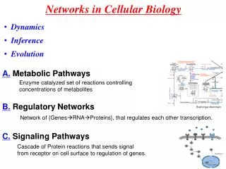
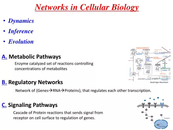
1. Networks in Cellular Biology • Dynamics • Inference • Evolution A. Metabolic Pathways Boehringer-Mannheim B. Regulatory Networks Enzyme catalyzed set of reactions controlling concentrations of metabolites Network of {GenesRNAProteins}, that regulates each other transcription. C. Signaling Pathways Cascade of Protein reactions that sends signal from receptor on cell surface to regulation of genes. Sreenath et al.(2008)

2. Networks  A Cell  A Human • A cell has ~1013 atoms. 1013 • Describing atomic behavior needs ~1015 time steps per second 1028 • A human has ~1013 cells. 1041 105 • Large descriptive networks have 103-105 edges, nodes and labels • What happened to the missing 36 orders of magnitude??? • Which approximations have been made? A Spatial homogeneity  103-107molecules can be represented by concentration ~104 B One molecule (104), one action per second (1015) ~1019 C Little explicit description beyond the cell ~1013 A Compartmentalisation can be added, some models (ie Turing) create spatial heterogeneity B Hopefully valid, but hard to test C Techniques (ie medical imaging) gather beyond cell data

3. Systems Biology versus Integrative Genomics Definitions: Systems Biology: Predictive Modelling of Biological Systems based on biochemical, physiological and molecular biological knowledge Integrative Genomics: Statistical Inference based on observations of G - genetic variation • Within species – population genetics • Between species – molecular evolution and comparative genomics T - transcript levels P - protein concentrations M - metabolite concentrations F – phenotype/phenome A few other data types available. Little biological knowledge beyond “gene” Integrative Genomics is more top-down and Systems Biology more bottom-up Prediction: Integrative Genomics and Systems Biology will converge!!

4. A repertoire of Dynamic Network Models To get to networks: No space heterogeneity  molecules are represented by numbers/concentrations Definition of Biochemical Network: • A set of k nodes (chemical species) labelled by kind and possibly concentrations, Xk. • A set of reactions/conservation laws (edges/hyperedges) is a set of nodes. Nodes can be labelled by numbers in reactions. If directed reactions, then an inset and an outset. • Description of dynamics for each rule. ODEs – ordinary differential equations 2 2 Mass Action 3 7 1 1 k Time Delay Discrete Deterministic – the reactions are applied. Boolean – only 0/1 values. Stochastic Discrete: the reaction fires after exponential with some intensity I(X1,X2) updating the number of molecules Continuous: the concentrations fluctuate according to a diffusion process.

5. Networks & Hypergraphs 26 2k 236 2k*k 26*5*4/3 2k*k-1*k-2/3 6 k 3 3 2 2 A E C D B F How many directed hypergraphs are there? 0’th order ? Constant removal/addition of a component 1st order ? Exponential growth/decay as function of some concentration 2nd order ? Pairwise collision creation: (A, B --> C) (no multiplicities) i-in, o-out ? Partition components into in-set, out-set, rest-set (no multiplicities) Arbitrary ? K. Gatermann, B. Huber: A family of sparse polynomial systems arising in chemical reaction systems. Journal of Symbolic Computation 33(3), 275-305, 2002

6. Number of Networks • undirected graphs • Connected undirected graphs • Directed Acyclic Graphs - DAGs • Interesting Problems to consider: • The size of neighborhood of a graph? • Given a set of subgraphs, who many graphs have them as subgraphs?

7. ODEs with Noise This can be modeled by Where Feed forward loop (FFL) Z X Y If noise is given a distribution the problem is well defined and statistical estimation can be done Data and estimation Goodness of Fit and Significance Objective is to estimate from noisy measurements of expression levels Cao and Zhao (2008) “Estimating Dynamic Models for gene regulation networks” Bioinformatics 24.14.1619-24

8. Gaussian Processes Definition: A Stochastic Process X(t) is a GP if all finite sets of time points, t1,t2,..,tk, defines stochastic variable that follows a multivariate Normal distribution, N(m,S), where m is the k-dimensional mean and S is the k*k dimensional covariance matrix. Examples: Brownian Motion: All increments are N( ,Dt) distributed. Dt is the time period for the increment. No equilibrium distribution. Ornstein-Uhlenbeck Process – diffusion process with centralizing linear drift. N( , ) as equilibrium distribution. One TF (transcription factor – black ball) (f(t)) whose concentration fluctuates over times influence k genes (xj) (four in this illustration) through their TFBS (transcription factor binding site - blue). The strength of its influence is described through a gene specific sensitivity, Sj. Dj– decay of gene j, Bj– production of gene j in absence of TF

9. Gaussian Processes Gaussian Processes are characterized by their mean and variances thus calculating these for xj and f at pairs of time, t and t’, points is a key objective Observable level Hidden and Gaussian time t t’ Correlation between two time points of f Correlation between two time points of same x’es Rattray, Lawrence et al. Manchester Correlation between two time points of different x’es Correlation between two time points of x and f This defines a prior on the observables Then observe and a posterior distribution is defined

10. Gaussian Processes Relevant Generalizations: Non-linear response function Multiple transcription factors Network relationship between genes Observations in Multiple Species Comments: Inference of Hidden Processes has strong similarity to genome annotation

11. Graphical Models Edges/Hyperedges – directed or undirected – determines the combined distribution on all nodes. Labeled Nodes: each associated a stochastic variable that can be observed or not. 2 2 1 1 3 3 4 4 • Conditional Independence • Gaussian • Correlation Graphs • Causality Graphs

12. Dynamic Bayesian Networks • Make a time series of of it • Model the observable as function of present network Take a graphical model Perrin et al. (2003) “Gene networks inference using dynamic Bayesian networks” Bioinformatics 19.suppl.138-48. Example: DNA repair Inference about the level of hidden variables can be made

13. Equation Discovery I • Given – Knowledge of System and Data: • Set of labeled quantities • Time Course Data for these quantities People: http://www-ai.ijs.si/~ljupco/http://cll.stanford.edu/~langley/ Software: http://kt.ijs.si/software/ciper/ http://www-ai.ijs.si/~ljupco/ed/lagrange.html • Given – Modeling and Inference • Natural Dynamics for the quantities • Optimization Criteria: Root Means Square, Likelihood, Bayesian Integration. • Dual Search Techniques: • Exhaustive or Heuristic Search • Standard Numerical Optimization • Dual Search Problem: • Discrete Search over Equation Structures • Estimating continuous parameters to fit data a[A], [A0], [B0],[C0]

14. Inference and Evolution B A D C Evolve B’ Infer network A’ D’ C’ Observe (data) Human Mouse

15. Suggestion: Evolving Dynamical Systems • Goal: a time reversible model with sparse mass action system of order three!! Adding/Deleting components (TKF91): Add rate: (k+1)l Delete rate: km Adding reactions with birth of component: There are 3k(k-1) possible reactions involving a new-born • Reaction Coefficients: • Continuous Time Continuous States Markov Process - specifically Diffusion. • For instance Ornstein-Uhlenbeck, which has Gausssian equilibrium distribution

16. Evolve! Network Example: Cell Cycle • What is the edit distance? • Which properties are conserved? • If you only knew Budding Yeast, how much would you know about Fission Yeast? • As N1 starts to evolve, you can only add reactions. Isn’t that strange? • On a path from N1 to N2 how close to the minimal has evolution travelled? • What is the number of equation systems possible for N1?